CMGFM: simulation

This vignette introduces the usage of CMGFM for the analysis of high-dimensional multimodality data with additional covariates, by comparison with other methods.

The package can be loaded with the command:

library(CMGFM)
#> Loading required package: irlba
#> Loading required package: Matrix
#> CMGFM :  Covariate-augumented generalized factor model is designed to account for cross-modal heterogeneity, capture nonlinear dependencies among the data, incorporate additional information, and provide excellent interpretability while maintaining high computational efficiency.

Generate the simulated data

First, we generate the data simulated data.

pveclist <- list('gaussian'=c(50, 150),'poisson'=c(50, 150),
                 'binomial'=c(100,60))
q <- 6
sigmavec <- rep(1,3)
pvec <- unlist(pveclist)
methodNames <- c("CMGFM", "GFM", "MRRR", "LFR" , "GPCA", "COAP")

datlist <- gendata_cmgfm(pveclist = pveclist, seed = 1, n = 300,d = 3,
                           q = q, rho = rep(1,length(pveclist)), rho_z=0.2,
                           sigmavec=sigmavec, sigma_eps=1)
str(datlist)
#> List of 12
#>  $ XList    :List of 3
#>   ..$ : num [1:300, 1:200] -0.412 3.69 -1.696 -1.371 2.124 ...
#>   .. ..- attr(*, "dimnames")=List of 2
#>   .. .. ..$ : NULL
#>   .. .. ..$ : NULL
#>   ..$ : int [1:300, 1:200] 0 5 0 0 7 1 0 0 0 1 ...
#>   ..$ : int [1:300, 1:160] 0 0 1 0 0 1 1 1 1 0 ...
#>  $ Z        : num [1:300, 1:3] 0.315 0.113 0.263 -0.259 -0.07 ...
#>  $ types    : chr [1:3] "gaussian" "poisson" "binomial"
#>  $ Alist    :List of 1
#>   ..$ : num [1:300, 1:6] 0 0 0 0 0 0 0 0 0 0 ...
#>  $ numvarmat: num [1:3, 1:2] 50 50 100 150 150 60
#>   ..- attr(*, "dimnames")=List of 2
#>   .. ..$ : chr [1:3] "gaussian" "poisson" "binomial"
#>   .. ..$ : NULL
#>  $ B0List   :List of 3
#>   ..$ :List of 2
#>   .. ..$ : num [1:50, 1:6] 0.2622 -0.6594 -0.0584 0.0826 -0.3536 ...
#>   .. ..$ : num [1:150, 1:6] 0.0729 -0.1236 -0.1994 0.7284 0.5208 ...
#>   ..$ :List of 2
#>   .. ..$ : num [1:50, 1:6] 0.322 -0.0678 0.0515 -0.1115 0.1911 ...
#>   .. ..$ : num [1:150, 1:6] 0.3414 -0.1357 -0.2816 -0.1411 0.0463 ...
#>   ..$ :List of 2
#>   .. ..$ : num [1:100, 1:6] 0.0114 -0.4359 0.1958 -0.3451 0.0457 ...
#>   .. ..$ : num [1:60, 1:6] 0.7305 -0.0567 0.2556 0.1347 0.3636 ...
#>  $ mu0List  :List of 3
#>   ..$ : num [1:200] 0.195 0.295 0.23 -0.122 0.605 ...
#>   ..$ : num [1:200] -0.46 0.108 -0.177 -0.211 -0.469 ...
#>   ..$ : num [1:160] -0.159 -0.312 0.214 0.46 -0.783 ...
#>  $ beta0List:List of 3
#>   ..$ : num [1:3, 1:2] -1.253 0.367 -1.671 3.191 0.659 ...
#>   ..$ : num [1:3, 1:2] 0.683 0.827 0.244 -3.179 -1.575 ...
#>   ..$ : num [1:3, 1:2] 3.0383 1.9234 -2.2854 -0.7993 0.0781 ...
#>  $ Uplist   :List of 3
#>   ..$ :List of 2
#>   .. ..$ : num [1:50, 1:7] 0.195 0.295 0.23 -0.122 0.605 ...
#>   .. ..$ : num [1:150, 1:7] -0.147 -0.418 0.228 -0.054 0.961 ...
#>   ..$ :List of 2
#>   .. ..$ : num [1:50, 1:7] -0.46 0.108 -0.177 -0.211 -0.469 ...
#>   .. ..$ : num [1:150, 1:7] 0.1795 0.0427 0.1158 0.3639 0.1529 ...
#>   ..$ :List of 2
#>   .. ..$ : num [1:100, 1:7] -0.159 -0.312 0.214 0.46 -0.783 ...
#>   .. ..$ : num [1:60, 1:7] 0.0809 -0.5117 -0.6635 -0.0317 -0.6377 ...
#>  $ U0List   :List of 3
#>   ..$ : num [1:300, 1:2] -0.626 0.184 -0.836 1.595 0.33 ...
#>   ..$ : num [1:300, 1:2] -0.626 0.184 -0.836 1.595 0.33 ...
#>   ..$ : num [1:300, 1:2] -0.626 0.184 -0.836 1.595 0.33 ...
#>  $ F0       : num [1:300, 1:6] -0.626 0.184 -0.836 1.595 0.33 ...
#>  $ sigma_eps: num 1
XList <- datlist$XList
Z <- datlist$Z
numvarmat <- datlist$numvarmat
Uplist <- list()
k <- 1
for(id in 1:length(datlist$Uplist)){
    for(im in 1:length(datlist$Uplist[[id]])){
      Uplist[[k]] <- datlist$Uplist[[id]][[im]]
      k <- k + 1
    }
}
types <- datlist$types

Fit the CMGFM model using the function CMGFM() in the R package CMGFM. Users can use ?CMGFM to see the details about this function

system.time({
  tic <- proc.time()
  rlist <- CMGFM(XList, Z, types=types, q=q, numvarmat=numvarmat)
  toc <- proc.time()
  time_smgfm <- toc[3] - tic[3]
})
#> iter = 2, ELBO= 1991125.056475, dELBO=1.000000 
#> iter = 3, ELBO= 2005063.871790, dELBO=0.007000 
#> iter = 4, ELBO= 2010542.767770, dELBO=0.002733 
#> iter = 5, ELBO= 2013223.740359, dELBO=0.001333 
#> iter = 6, ELBO= 2014945.775650, dELBO=0.000855 
#> iter = 7, ELBO= 2016228.099702, dELBO=0.000636 
#> iter = 8, ELBO= 2017258.673090, dELBO=0.000511 
#> iter = 9, ELBO= 2018123.186985, dELBO=0.000429 
#> iter = 10, ELBO= 2018867.740559, dELBO=0.000369 
#> iter = 11, ELBO= 2019520.570983, dELBO=0.000323 
#> iter = 12, ELBO= 2020100.677428, dELBO=0.000287 
#> iter = 13, ELBO= 2020621.729760, dELBO=0.000258 
#> iter = 14, ELBO= 2021094.053165, dELBO=0.000234 
#> iter = 15, ELBO= 2021525.743440, dELBO=0.000214 
#> iter = 16, ELBO= 2021923.351548, dELBO=0.000197 
#> iter = 17, ELBO= 2022292.338348, dELBO=0.000182 
#> iter = 18, ELBO= 2022637.400259, dELBO=0.000171 
#> iter = 19, ELBO= 2022962.720218, dELBO=0.000161 
#> iter = 20, ELBO= 2023272.171344, dELBO=0.000153 
#> iter = 21, ELBO= 2023569.470842, dELBO=0.000147 
#> iter = 22, ELBO= 2023858.213468, dELBO=0.000143 
#> iter = 23, ELBO= 2024141.525295, dELBO=0.000140 
#> iter = 24, ELBO= 2024420.678070, dELBO=0.000138 
#> iter = 25, ELBO= 2024692.109344, dELBO=0.000134 
#> iter = 26, ELBO= 2024946.637220, dELBO=0.000126 
#> iter = 27, ELBO= 2025178.764916, dELBO=0.000115 
#> iter = 28, ELBO= 2025392.822741, dELBO=0.000106 
#> iter = 29, ELBO= 2025594.259740, dELBO=0.000099 
#> iter = 30, ELBO= 2025785.510378, dELBO=0.000094
#>    user  system elapsed 
#>    0.03    0.00    0.28

Check the increased property of the evidence lower bound function.

library(ggplot2)
dat_iter <- data.frame(iter=1:length(rlist$ELBO_seq), ELBO=rlist$ELBO_seq)
ggplot(data=dat_iter, aes(x=iter, y=ELBO)) + geom_line() + geom_point() + theme_bw(base_size = 20)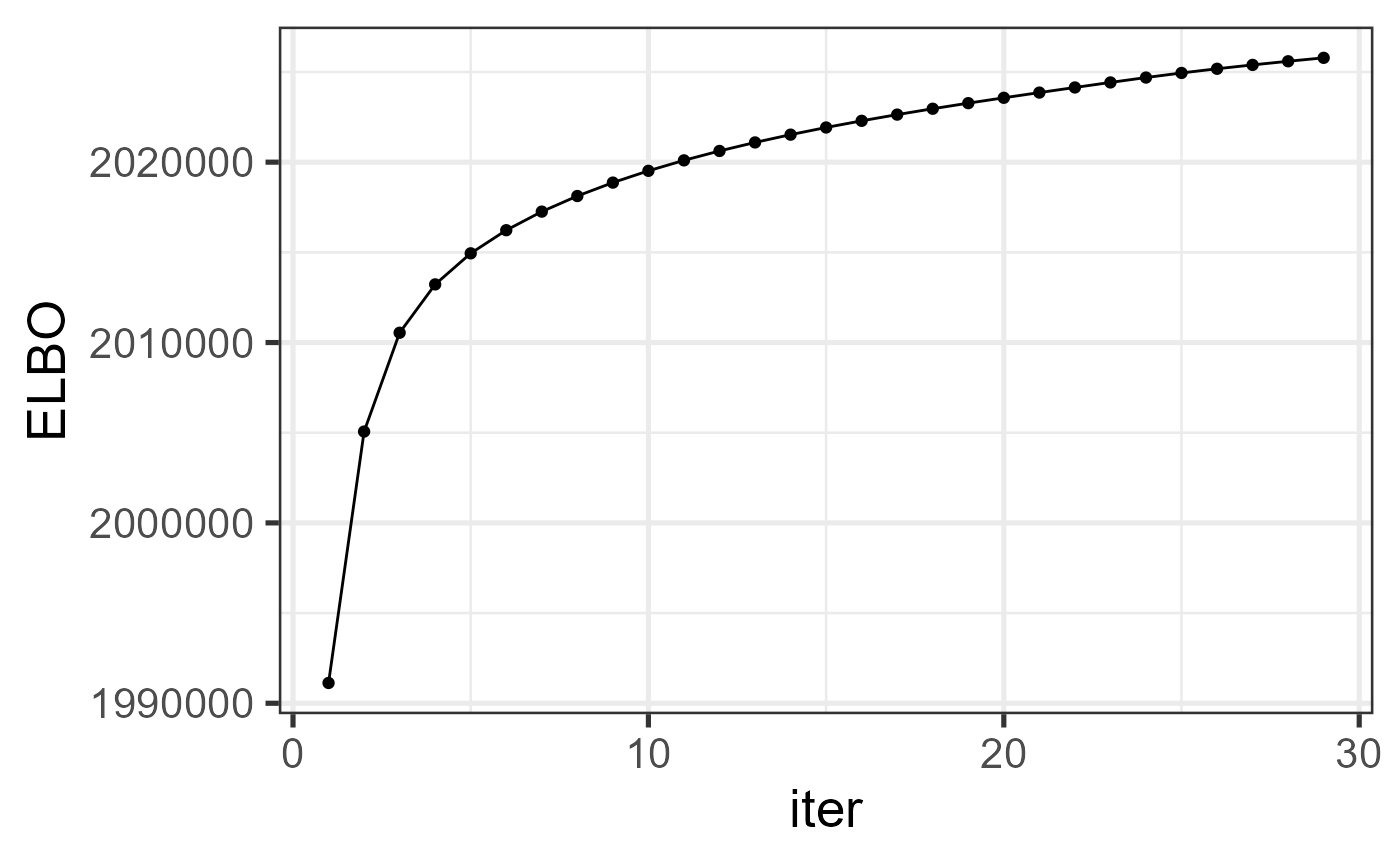

We calculate the metrics to measure the estimation accuracy, where the trace statistic is used to measure the estimation accuracy of loading matrix and prediction accuracy of factor matrix, which is evaluated by the function measurefun() in the R package GFM, and the root of mean square error is adopted to measure the estimation error of bbeta.

library(GFM)
#> Loading required package: doSNOW
#> Loading required package: foreach
#> Loading required package: iterators
#> Loading required package: snow
#> Loading required package: parallel
#> 
#> Attaching package: 'parallel'
#> The following objects are masked from 'package:snow':
#> 
#>     closeNode, clusterApply, clusterApplyLB, clusterCall, clusterEvalQ,
#>     clusterExport, clusterMap, clusterSplit, makeCluster, parApply,
#>     parCapply, parLapply, parRapply, parSapply, recvData, recvOneData,
#>     sendData, splitIndices, stopCluster
#> GFM :  Generalized factor model is implemented for ultra-high dimensional data with mixed-type variables.
#> Two algorithms, variational EM and alternate maximization, are designed to implement the generalized factor model,
#> respectively. The factor matrix and loading matrix together with the number of factors can be well estimated.
#> This model can be employed in social and behavioral sciences, economy and finance, and  genomics,
#> to extract interpretable nonlinear factors. More details can be referred to
#> Wei Liu, Huazhen Lin, Shurong Zheng and Jin Liu. (2021) <doi:10.1080/01621459.2021.1999818>.   Check out our Package website (https://feiyoung.github.io/GFM/docs/index.html) for a more complete description of the methods and analyses
hUplist <- lapply(seq_along(rlist$Bf), function(m) cbind(rlist$muf[[m]], rlist$Bf[[m]]))
metricList <- list()
metricList$CMGFM <- list()
meanTr <- function(hBlist, Blist,  type='trace_statistic'){
  ###It is noted that the trace statistics is not symmetric, the true value must be in last
  trvec <- sapply(1:length(Blist), function(j) measurefun(hBlist[[j]], Blist[[j]], type = type))
  return(mean(trvec))
}
normvec <- function(x) sqrt(sum(x^2/ length(x)))
metricList$CMGFM$Tr_F <- measurefun(rlist$M, datlist$F0)
metricList$CMGFM$Tr_Upsilon <- meanTr(hUplist, Uplist)
metricList$CMGFM$Tr_U <- measurefun(Reduce(cbind,rlist$Xif), Reduce(cbind, datlist$U0))
metricList$CMGFM$beta_norm <- normvec(as.vector(Reduce(cbind,rlist$betaf)- Reduce(cbind,datlist$beta0List)))
metricList$CMGFM$Time <- rlist$time_use

Compare with other methods

We compare CMGFM with various prominent methods in the literature. They are (1) High-dimensional LFM (Bai and Ng 2002) implemented in the R package GFM; (2) PoissonPCA (Kenney et al. 2021) implemented in the R package PoissonPCA; (3) Zero-inflated Poisson factor model (ZIPFA, Xu et al. 2021) implemented in the R package ZIPFA; (4) Generalized factor model (Liu et al. 2023) implemented in the R package GFM; (5) PLNPCA (Chiquet et al. 2018) implemented in the R package PLNmodels; (6) Generalized Linear Latent Variable Models (GLLVM, Hui et al. 2017) implemented in the R package gllvm. (7) Poisson regression model for each \(x_{ij}, (j = 1,··· ,p)\), implemented in stats R package; (8) Multi-response reduced-rank Poisson regression model (MMMR, Luo et al. 2018) implemented in rrpack R package.

(1). First, we implemented the generalized factor model (LFM) and record the metrics that measure the estimation accuracy and computational cost.

metricList$GFM <- list()
tic <- proc.time()
res_gfm <- gfm(XList, types=types, q=q)
#> Starting the two-step method with varitional EM in the first step...
#> iter = 2, ELBO= 2697769.202257, dELBO=1.000000 
#> iter = 3, ELBO= 2702423.237715, dELBO=0.001725 
#> iter = 4, ELBO= 2704625.687731, dELBO=0.000815 
#> iter = 5, ELBO= 2705737.853138, dELBO=0.000411 
#> iter = 6, ELBO= 2706272.269271, dELBO=0.000198 
#> iter = 7, ELBO= 2706482.230846, dELBO=0.000078
#> Finish the two-step method
toc <- proc.time()
time_gfm <- toc[3] - tic[3]
mat2list <- function(B, pvec, by_row=TRUE){
  Blist <- list()
  pcum = c(0, cumsum(pvec))
  for(i in 1:length(pvec)){
    if(by_row){
      Blist[[i]] <- B[(pcum[i]+1):pcum[i+1],]
    }else{
      Blist[[i]] <- B[, (pcum[i]+1):pcum[i+1]]
    }
  }
  return(Blist)
}
metricList$GFM$Tr_F <- measurefun(res_gfm$hH, datlist$F0)
metricList$GFM$Tr_Upsilon <- meanTr(mat2list(cbind(res_gfm$hmu,res_gfm$hB), pvec), Uplist)
metricList$GFM$Tr_U <- NA
metricList$GFM$beta_norm <- NA
metricList$GFM$Time <- time_gfm

Eightly, we implemented the first version of multi-response reduced-rank Poisson regression model (MMMR, Luo et al. 2018) implemented in rrpack R package (MRRR-Z), that did not consider the latent factor structure but only the covariates.

mrrr_run <- function(Y, Z, numvarmat, rank0,family=list(poisson()),
                     familygroup,  epsilon = 1e-4, sv.tol = 1e-2,
                     lambdaSVD=0.1, maxIter = 2000, trace=TRUE, trunc=500){
  # epsilon = 1e-4; sv.tol = 1e-2; maxIter = 30; trace=TRUE,lambdaSVD=0.1
  Diag <- function(vec){
  q <- length(vec)
  if(q > 1){
    y <- diag(vec)
  }else{
    y <- matrix(vec, 1,1)
  }
  return(y)
}
  require(rrpack)
  q <- rank0
  n <- nrow(Y); p <- ncol(Y)
  X <- cbind(cbind(1, Z),  diag(n))
  d <- ncol(Z)
  ## Trunction
  Y[Y>trunc] <- trunc
  Y[Y< -trunc] <- -trunc
  
  tic <- proc.time()
  pvec <- as.vector(t(numvarmat))
  pvec <- pvec[pvec>0]
  pcums <- cumsum(pvec)
  idxlist <- list()
  idxlist[[1]] <- 1:pcums[1]
  if(length(pvec)>1){
    for(i in 2:length(pvec)){
      idxlist[[i]] <- (pcums[i-1]+1):pcums[i] 
    }
  }
  
  svdX0d1 <- svd(X)$d[1]
  init1 = list(kappaC0 = svdX0d1 * 5)
  offset = NULL
  control = list(epsilon = epsilon, sv.tol = sv.tol, maxit = maxIter,
                 trace = trace, gammaC0 = 1.1, plot.cv = TRUE,
                 conv.obj = TRUE)
  res_mrrr <- mrrr(Y=Y, X=X[,-1], family = family, familygroup = familygroup,
                   penstr = list(penaltySVD = "rankCon", lambdaSVD = lambdaSVD),
                   control = control, init = init1, maxrank = rank0+d) #
  
  hmu <- res_mrrr$coef[1,]
  hbeta <- t(res_mrrr$coef[2:(d+1),])
  hTheta <- res_mrrr$coef[-c(1:(d+1)),]
  
  hbeta_rf <- NULL
  for(i in seq_along(pvec)){
    hbeta_rf <- cbind(hbeta_rf, colMeans(hbeta[idxlist[[i]],]))
  }
  
  # Matrix::rankMatrix(hTheta)
  svd_Theta <- svd(hTheta, nu=q, nv=q)
  hH <- svd_Theta$u
  hB <- svd_Theta$v %*% Diag(svd_Theta$d[1:q])
  toc <- proc.time()
  time_mrrr <- toc[3] - tic[3]
  
  return(list(hH=hH, hB=hB, hmu= hmu, beta=hbeta_rf, time_use=time_mrrr))
}

family_use <- list(gaussian(), poisson(), binomial())
familygroup <- sapply(seq_along(datlist$XList), function(j) rep(j, ncol(datlist$XList[[j]])))
res_mrrr <- mrrr_run(Reduce(cbind, datlist$XList),  Z = Z, numvarmat, rank0=q, family=family_use,
                       familygroup = unlist(familygroup), maxIter=100) #
#> Loading required package: rrpack
#> iter =  1  obj/Cnorm_diff =  2285754  
#> iter =  2  obj/Cnorm_diff =  1895923  
#> iter =  3  obj/Cnorm_diff =  1602853  
#> iter =  4  obj/Cnorm_diff =  1327399  
#> iter =  5  obj/Cnorm_diff =  1131392  
#> iter =  6  obj/Cnorm_diff =  1013997  
#> iter =  7  obj/Cnorm_diff =  938923.5  
#> iter =  8  obj/Cnorm_diff =  880858.6  
#> iter =  9  obj/Cnorm_diff =  831925.5  
#> iter =  10  obj/Cnorm_diff =  788683.1  
#> iter =  11  obj/Cnorm_diff =  755306  
#> iter =  11  obj/Cnorm_diff =  755306  
#> iter =  12  obj/Cnorm_diff =  731040.1  
#> iter =  13  obj/Cnorm_diff =  720962.6  
#> iter =  14  obj/Cnorm_diff =  714250.6  
#> iter =  15  obj/Cnorm_diff =  708120.1  
#> iter =  16  obj/Cnorm_diff =  701718.5  
#> iter =  17  obj/Cnorm_diff =  694597.2  
#> iter =  18  obj/Cnorm_diff =  687113.1  
#> iter =  19  obj/Cnorm_diff =  678866.8  
#> iter =  20  obj/Cnorm_diff =  670110.7  
#> iter =  21  obj/Cnorm_diff =  660703.3  
#> iter =  22  obj/Cnorm_diff =  650862.2  
#> iter =  23  obj/Cnorm_diff =  640609.7  
#> iter =  23  obj/Cnorm_diff =  640609.7  
#> iter =  24  obj/Cnorm_diff =  634136.5  
#> iter =  25  obj/Cnorm_diff =  630295.3  
#> iter =  26  obj/Cnorm_diff =  628296.4  
#> iter =  27  obj/Cnorm_diff =  626027.9  
#> iter =  28  obj/Cnorm_diff =  623654.6  
#> iter =  29  obj/Cnorm_diff =  620954.6  
#> iter =  30  obj/Cnorm_diff =  618049.5  
#> iter =  31  obj/Cnorm_diff =  614697.6  
#> iter =  32  obj/Cnorm_diff =  610953.2  
#> iter =  33  obj/Cnorm_diff =  606644  
#> iter =  34  obj/Cnorm_diff =  601733.5  
#> iter =  34  obj/Cnorm_diff =  601733.5  
#> iter =  35  obj/Cnorm_diff =  596206.5  
#> iter =  36  obj/Cnorm_diff =  595329.2  
#> iter =  37  obj/Cnorm_diff =  594390.1  
#> iter =  38  obj/Cnorm_diff =  593270.4  
#> iter =  39  obj/Cnorm_diff =  591937.5  
#> iter =  40  obj/Cnorm_diff =  590355.4  
#> iter =  41  obj/Cnorm_diff =  588483.5  
#> iter =  42  obj/Cnorm_diff =  586277.2  
#> iter =  43  obj/Cnorm_diff =  583688  
#> iter =  44  obj/Cnorm_diff =  580665.3  
#> iter =  45  obj/Cnorm_diff =  577158.2  
#> iter =  46  obj/Cnorm_diff =  573119.8  
#> iter =  47  obj/Cnorm_diff =  568520.9  
#> iter =  47  obj/Cnorm_diff =  568520.9  
#> iter =  48  obj/Cnorm_diff =  563522.6  
#> iter =  49  obj/Cnorm_diff =  562940.9  
#> iter =  50  obj/Cnorm_diff =  562299.2  
#> iter =  51  obj/Cnorm_diff =  561541.1  
#> iter =  52  obj/Cnorm_diff =  560644.4  
#> iter =  53  obj/Cnorm_diff =  559586.9  
#> iter =  54  obj/Cnorm_diff =  558340.3  
#> iter =  55  obj/Cnorm_diff =  556872.3  
#> iter =  56  obj/Cnorm_diff =  555143.8  
#> iter =  57  obj/Cnorm_diff =  553109.6  
#> iter =  58  obj/Cnorm_diff =  550720.4  
#> iter =  59  obj/Cnorm_diff =  547934.6  
#> iter =  60  obj/Cnorm_diff =  544813.2  
#> iter =  60  obj/Cnorm_diff =  544813.2  
#> iter =  61  obj/Cnorm_diff =  543904.5  
#> iter =  62  obj/Cnorm_diff =  542573.5  
#> iter =  63  obj/Cnorm_diff =  541631.6  
#> iter =  64  obj/Cnorm_diff =  540700.3  
#> iter =  65  obj/Cnorm_diff =  539689  
#> iter =  66  obj/Cnorm_diff =  538625.6  
#> iter =  67  obj/Cnorm_diff =  537504.6  
#> iter =  68  obj/Cnorm_diff =  536307  
#> iter =  69  obj/Cnorm_diff =  534984.4  
#> iter =  70  obj/Cnorm_diff =  533467.5  
#> iter =  71  obj/Cnorm_diff =  531678.1  
#> iter =  72  obj/Cnorm_diff =  529609.3  
#> iter =  72  obj/Cnorm_diff =  529609.3  
#> iter =  73  obj/Cnorm_diff =  527865.5  
#> iter =  74  obj/Cnorm_diff =  527373.4  
#> iter =  75  obj/Cnorm_diff =  526906.6  
#> iter =  76  obj/Cnorm_diff =  526374.9  
#> iter =  77  obj/Cnorm_diff =  525761.6  
#> iter =  78  obj/Cnorm_diff =  525061.1  
#> iter =  79  obj/Cnorm_diff =  524258.2  
#> iter =  80  obj/Cnorm_diff =  523338.7  
#> iter =  81  obj/Cnorm_diff =  522276  
#> iter =  82  obj/Cnorm_diff =  521034.1  
#> iter =  83  obj/Cnorm_diff =  519565  
#> iter =  84  obj/Cnorm_diff =  517836.7  
#> iter =  85  obj/Cnorm_diff =  516024.2  
#> iter =  85  obj/Cnorm_diff =  516024.2  
#> iter =  85  obj/Cnorm_diff =  516024.2  
#> iter =  85  obj/Cnorm_diff =  516024.2  
#> iter =  85  obj/Cnorm_diff =  516024.2  
#> iter =  85  obj/Cnorm_diff =  516024.2  
#> iter =  85  obj/Cnorm_diff =  516024.2

metricList$MRRR <- list()
metricList$MRRR$Tr_F <- measurefun(res_mrrr$hH, datlist$F0)
metricList$MRRR$Tr_Upsilon <-meanTr(mat2list(cbind(res_mrrr$hmu,res_mrrr$hB), pvec), Uplist)
metricList$MRRR$Tr_U <-NA
metricList$MRRR$beta_norm <- normvec(as.vector(res_mrrr$beta- Reduce(cbind,datlist$beta0List)))
metricList$MRRR$Time <- res_mrrr$time_use

Visualize the comparison of performance

Next, we summarized the metrics for COAP and other compared methods in a dataframe object.

list2vec <- function(xlist){
  nn <- length(xlist)
  me <- rep(NA, nn)
  idx_noNA <- which(sapply(xlist, function(x) !is.null(x)))
  for(r in idx_noNA) me[r] <- xlist[[r]]
  return(me)
}

dat_metric <- data.frame(Tr_F = sapply(metricList, function(x) x$Tr_F), 
                         Tr_Upsilon = sapply(metricList, function(x) x$Tr_Upsilon),
                         Tr_U = sapply(metricList, function(x) x$Tr_U),
                         beta_norm =sapply(metricList, function(x) x$beta_norm),
                         Time = sapply(metricList, function(x) x$Time),
                         Method = names(metricList))
dat_metric
#>            Tr_F Tr_Upsilon      Tr_U beta_norm  Time Method
#> CMGFM 0.9935940  0.7785991 0.9644858 0.8201792  0.28  CMGFM
#> GFM   0.6829262  0.7051994        NA        NA  0.62    GFM
#> MRRR  0.3629987  0.5669866        NA 1.3579832 23.30   MRRR

Plot the results for COAP and other methods, which suggests that CMGFM achieves better estimation accuracy for the quantities of interest.

library(cowplot)
p1 <- ggplot(data=subset(dat_metric, !is.na(Tr_F)), aes(x= Method, y=Tr_F, fill=Method)) + geom_bar(stat="identity") + xlab(NULL) + scale_x_discrete(breaks=NULL) + theme_bw(base_size = 16)
p2 <- ggplot(data=subset(dat_metric, !is.na(Tr_Upsilon)), aes(x= Method, y=Tr_Upsilon, fill=Method)) + geom_bar(stat="identity") + xlab(NULL) + scale_x_discrete(breaks=NULL)+ theme_bw(base_size = 16)
p3 <- ggplot(data=subset(dat_metric, !is.na(beta_norm)), aes(x= Method, y=beta_norm, fill=Method)) + geom_bar(stat="identity") + xlab(NULL) + scale_x_discrete(breaks=NULL)+ theme_bw(base_size = 16)
p4 <- ggplot(data=subset(dat_metric, !is.na(Time)), aes(x= Method, y=Time, fill=Method)) + geom_bar(stat="identity") + xlab(NULL) + scale_x_discrete(breaks=NULL)+ theme_bw(base_size = 16)
plot_grid(p1,p2,p3, p4, nrow=2, ncol=2)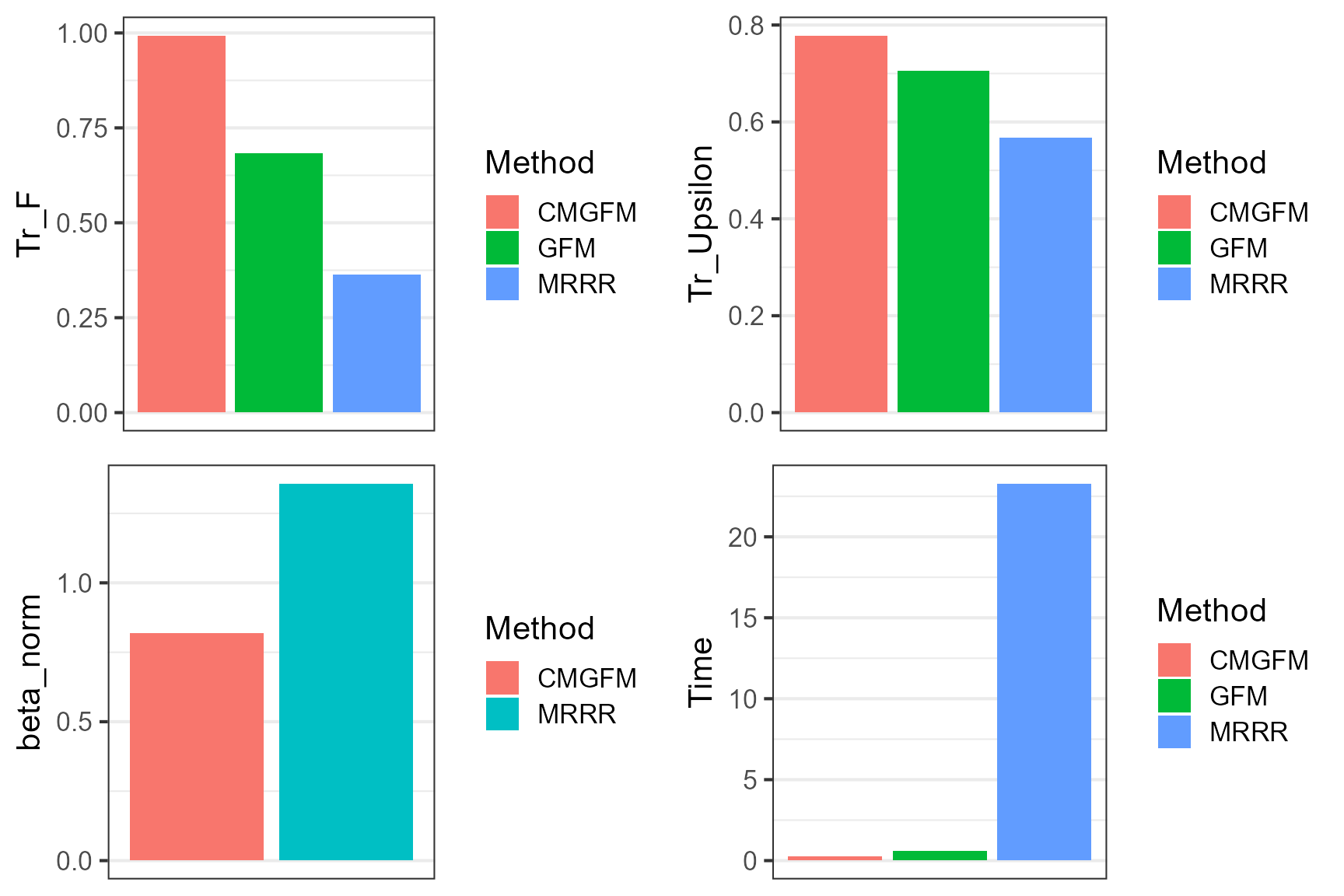

Select the parameters

We applied the maximum singular value ratio based method to select the number of factors. The results showed that the maximum SVR method has the potential to identify the true values.


hq <- MSVR(XList, Z, types=types, numvarmat, q_max=20)
#> iter = 2, ELBO= 1996035.425921, dELBO=1.000000 
#> iter = 3, ELBO= 2008870.623908, dELBO=0.006430 
#> iter = 4, ELBO= 2013435.986180, dELBO=0.002273 
#> iter = 5, ELBO= 2015986.295861, dELBO=0.001267 
#> iter = 6, ELBO= 2017732.453117, dELBO=0.000866 
#> iter = 7, ELBO= 2019070.938978, dELBO=0.000663 
#> iter = 8, ELBO= 2020159.319418, dELBO=0.000539 
#> iter = 9, ELBO= 2021075.256204, dELBO=0.000453 
#> iter = 10, ELBO= 2021863.403668, dELBO=0.000390 
#> iter = 11, ELBO= 2022552.576503, dELBO=0.000341 
#> iter = 12, ELBO= 2023162.855216, dELBO=0.000302 
#> iter = 13, ELBO= 2023708.974155, dELBO=0.000270 
#> iter = 14, ELBO= 2024202.153249, dELBO=0.000244 
#> iter = 15, ELBO= 2024651.196115, dELBO=0.000222 
#> iter = 16, ELBO= 2025063.200205, dELBO=0.000203 
#> iter = 17, ELBO= 2025444.043705, dELBO=0.000188 
#> iter = 18, ELBO= 2025798.738205, dELBO=0.000175 
#> iter = 19, ELBO= 2026131.699768, dELBO=0.000164 
#> iter = 20, ELBO= 2026446.968622, dELBO=0.000156 
#> iter = 21, ELBO= 2026748.383268, dELBO=0.000149 
#> iter = 22, ELBO= 2027039.661075, dELBO=0.000144 
#> iter = 23, ELBO= 2027324.185988, dELBO=0.000140 
#> iter = 24, ELBO= 2027603.938867, dELBO=0.000138 
#> iter = 25, ELBO= 2027876.769478, dELBO=0.000135 
#> iter = 26, ELBO= 2028134.194499, dELBO=0.000127 
#> iter = 27, ELBO= 2028368.473987, dELBO=0.000116 
#> iter = 28, ELBO= 2028582.177694, dELBO=0.000105 
#> iter = 29, ELBO= 2028781.486569, dELBO=0.000098 
#> iter = 30, ELBO= 2028969.592915, dELBO=0.000093

print(c(q_true=q, q_est=hq))
#> q_true  q_est 
#>      6      6

Session Info

sessionInfo()
#> R version 4.4.0 (2024-04-24 ucrt)
#> Platform: x86_64-w64-mingw32/x64
#> Running under: Windows 11 x64 (build 22631)
#> 
#> Matrix products: default
#> 
#> 
#> locale:
#> [1] LC_COLLATE=Chinese (Simplified)_China.utf8 
#> [2] LC_CTYPE=Chinese (Simplified)_China.utf8   
#> [3] LC_MONETARY=Chinese (Simplified)_China.utf8
#> [4] LC_NUMERIC=C                               
#> [5] LC_TIME=Chinese (Simplified)_China.utf8    
#> 
#> time zone: Asia/Shanghai
#> tzcode source: internal
#> 
#> attached base packages:
#> [1] parallel  stats     graphics  grDevices utils     datasets  methods  
#> [8] base     
#> 
#> other attached packages:
#>  [1] cowplot_1.1.3    rrpack_0.1-13    GFM_1.2.1        doSNOW_1.0.20   
#>  [5] snow_0.4-4       iterators_1.0.14 foreach_1.5.2    ggplot2_3.5.1   
#>  [9] CMGFM_1.1        irlba_2.3.5.1    Matrix_1.7-0    
#> 
#> loaded via a namespace (and not attached):
#>  [1] sass_0.4.9        utf8_1.2.4        generics_0.1.3    shape_1.4.6.1    
#>  [5] lattice_0.22-6    digest_0.6.35     magrittr_2.0.3    evaluate_0.23    
#>  [9] grid_4.4.0        fastmap_1.1.1     glmnet_4.1-8      jsonlite_1.8.8   
#> [13] survival_3.5-8    purrr_1.0.2       fansi_1.0.6       scales_1.3.0     
#> [17] codetools_0.2-20  textshaping_0.3.7 jquerylib_0.1.4   cli_3.6.2        
#> [21] rlang_1.1.3       splines_4.4.0     munsell_0.5.1     withr_3.0.0      
#> [25] cachem_1.0.8      yaml_2.3.8        tools_4.4.0       memoise_2.0.1    
#> [29] dplyr_1.1.4       colorspace_2.1-0  vctrs_0.6.5       R6_2.5.1         
#> [33] lifecycle_1.0.4   fs_1.6.4          htmlwidgets_1.6.4 MASS_7.3-60.2    
#> [37] ragg_1.3.1        pkgconfig_2.0.3   desc_1.4.3        pkgdown_2.0.9    
#> [41] bslib_0.7.0       pillar_1.9.0      gtable_0.3.5      glue_1.7.0       
#> [45] Rcpp_1.0.12       systemfonts_1.0.6 highr_0.10        tidyselect_1.2.1 
#> [49] xfun_0.43         tibble_3.2.1      rstudioapi_0.16.0 knitr_1.46       
#> [53] farver_2.1.1      htmltools_0.5.8.1 labeling_0.4.3    rmarkdown_2.26   
#> [57] compiler_4.4.0

Wei Liu

2024-06-23

Generate the simulated data

Compare with other methods

Visualize the comparison of performance

Select the parameters