This vignette introduces the usage of COAP for the analysis of high-dimensional count data with additional high-dimensional covariates, by comparison with other methods.
The package can be loaded with the command:
library(COAP)
library(GFM)
#> Loading required package: doSNOW
#> Loading required package: foreach
#> Loading required package: iterators
#> Loading required package: snow
#> Loading required package: parallel
#>
#> Attaching package: 'parallel'
#> The following objects are masked from 'package:snow':
#>
#>     clusterApply, clusterApplyLB, clusterCall, clusterEvalQ,
#>     clusterExport, clusterMap, clusterSplit, makeCluster, parApply,
#>     parCapply, parLapply, parRapply, parSapply, splitIndices,
#>     stopCluster
#> GFM :  Generalized factor model is implemented for ultra-high dimensional data with mixed-type variables.
#> Two algorithms, variational EM and alternate maximization, are designed to implement the generalized factor model,
#> respectively. The factor matrix and loading matrix together with the number of factors can be well estimated.
#> This model can be employed in social and behavioral sciences, economy and finance, and  genomics,
#> to extract interpretable nonlinear factors. More details can be referred to
#> Wei Liu, Huazhen Lin, Shurong Zheng and Jin Liu. (2021) <doi:10.1080/01621459.2021.1999818>.   Check out our Package website (https://feiyoung.github.io/GFM/docs/index.html) for a more complete description of the methods and analyses
Generate the simulated data
First, we generate the data simulated data.
n <- 200; p <- 200;
d= 50
rank0 <- 6;
q = 5;
datList <- gendata_simu(seed = 1, n=n, p=p, d= d, rank0 = rank0, q= q, rho=c(2, 2),
                        sigma2_eps = 1)
#> Loading required package: MASS
X_count <- datList$X; Z <- datList$Z
H0 <- datList$H0; B0 <- datList$B0
bbeta0 <- cbind( datList$mu0, datList$bbeta0)
Fit the COAP model using the function RR_COAP() in the R package COAP. Users can use ?RR_COAP to see the details about this function
hq <- 5; hr <- 6
system.time({
  tic <- proc.time()
  reslist <- RR_COAP(X_count, Z= Z, q=hq, rank_use= hr, epsELBO = 1e-6)
  toc <- proc.time()
  time_coap <- toc[3] - tic[3]
})
#> Calculate initial values...
#> Loading required package: irlba
#> Loading required package: Matrix
#> iter = 2, ELBO= 311531.420000, dELBO=1.000145
#> iter = 3, ELBO= 316042.737970, dELBO=0.014481
#> iter = 4, ELBO= 317869.490388, dELBO=0.005780
#> iter = 5, ELBO= 318776.120476, dELBO=0.002852
#> iter = 6, ELBO= 319290.972752, dELBO=0.001615
#> iter = 7, ELBO= 319611.373938, dELBO=0.001003
#> iter = 8, ELBO= 319824.015899, dELBO=0.000665
#> iter = 9, ELBO= 319971.850666, dELBO=0.000462
#> iter = 10, ELBO= 320078.245025, dELBO=0.000333
#> iter = 11, ELBO= 320156.887531, dELBO=0.000246
#> iter = 12, ELBO= 320216.278565, dELBO=0.000186
#> iter = 13, ELBO= 320261.942528, dELBO=0.000143
#> iter = 14, ELBO= 320297.599344, dELBO=0.000111
#> iter = 15, ELBO= 320325.824786, dELBO=0.000088
#> iter = 16, ELBO= 320348.442910, dELBO=0.000071
#> iter = 17, ELBO= 320366.769724, dELBO=0.000057
#> iter = 18, ELBO= 320381.769961, dELBO=0.000047
#> iter = 19, ELBO= 320394.160880, dELBO=0.000039
#> iter = 20, ELBO= 320404.482598, dELBO=0.000032
#> iter = 21, ELBO= 320413.146652, dELBO=0.000027
#> iter = 22, ELBO= 320420.470080, dELBO=0.000023
#> iter = 23, ELBO= 320426.699664, dELBO=0.000019
#> iter = 24, ELBO= 320432.029390, dELBO=0.000017
#> iter = 25, ELBO= 320436.613167, dELBO=0.000014
#> iter = 26, ELBO= 320440.574186, dELBO=0.000012
#> iter = 27, ELBO= 320444.011876, dELBO=0.000011
#> iter = 28, ELBO= 320447.007121, dELBO=0.000009
#> iter = 29, ELBO= 320449.626207, dELBO=0.000008
#> iter = 30, ELBO= 320451.923844, dELBO=0.000007
#>    user  system elapsed
#>    0.09    0.01    0.75
Check the increased property of the envidence lower bound function.
library(ggplot2)
#> Warning: package 'ggplot2' was built under R version 4.1.3
dat_iter <- data.frame(iter=1:length(reslist$ELBO_seq), ELBO=reslist$ELBO_seq)
ggplot(data=dat_iter, aes(x=iter, y=ELBO)) + geom_line() + geom_point() + theme_bw(base_size = 20)
We calculate the metrics to measure the estimatioin accuracy, where the trace statistic is used to measure the estimation accuracy of loading matrix and prediction accuracy of factor matrix, which is evaluated by the function measurefun() in the R package GFM, and the root of mean square error is adopted to measure the estimation error of bbeta.
library(GFM)
metricList <- list()
metricList$COAP <- list()
metricList$COAP$Tr_H <- measurefun(reslist$H, H0)
metricList$COAP$Tr_B <- measurefun(reslist$B, B0)

norm_vec <- function(x) sqrt(sum(x^2/ length(x)))
metricList$COAP$err_bb <- norm_vec(reslist$bbeta-bbeta0)
metricList$COAP$err_bb1 <- norm_vec(reslist$bbeta[,1]-bbeta0[,1])
metricList$COAP$Time <- time_coap
Compare with other methods
We compare COAP with various prominent methods in the literature. They are (1) High-dimensional LFM (Bai and Ng 2002) implemented in the R package GFM; (2) PoissonPCA (Kenney et al. 2021) implemented in the R package PoissonPCA; (3) Zero-inflated Poisson factor model (ZIPFA, Xu et al. 2021) implemented in the R package ZIPFA; (4) Generalized factor model (Liu et al. 2023) implemented in the R package GFM; (5) PLNPCA (Chiquet et al. 2018) implemented in the R package PLNmodels; (6) Generalized Linear Latent Variable Models (GLLVM, Hui et al. 2017) implemented in the R package gllvm. (7) Poisson regression model for each \(x_{ij}, (j = 1,··· ,p)\), implemented in stats R package; (8) Multi-response reduced-rank Poisson regression model (MMMR, Luo et al. 2018) implemented in rrpack R package.
(1). First, we implemented the linear factor model (LFM) and record the metrics that measure the estimation accuracy and computational cost.
metricList$LFM <- list()
tic <- proc.time()
fit_lfm <- Factorm(X_count, q=q)
toc <- proc.time()
time_lfm <- toc[3] - tic[3]

hbb1 <- colMeans(X_count)
metricList$LFM$Tr_H <- measurefun(fit_lfm$hH, H0)
metricList$LFM$Tr_B <- measurefun(fit_lfm$hB, B0)
metricList$LFM$err_bb1 <- norm_vec(hbb1- bbeta0[,1])
metricList$LFM$err_bb <- NA
metricList$LFM$Time <- time_lfm
(2). Then, we implemented PoissonPCA and recorded the metrics.
metricList$PoissonPCA <- list()
library(PoissonPCA)
tic <- proc.time()
fit_poispca <- Poisson_Corrected_PCA(X_count, k= hq)
#> Warning in sqrt(eig$values): NaNs produced
toc <- proc.time()
time_ppca <- toc[3] - tic[3]

hbb1 <- colMeans(X_count)
metricList$PoissonPCA$Tr_H <- measurefun(fit_poispca$scores, H0)
metricList$PoissonPCA$Tr_B <- measurefun(fit_poispca$loadings, B0)
metricList$PoissonPCA$err_bb1 <- norm_vec(log(1+fit_poispca$center)- bbeta0[,1])
metricList$PoissonPCA$err_bb <- NA
metricList$PoissonPCA$Time <- time_ppca- Thirdly, we implemented the zero-inflated Poisson factor model:
## ZIPFA runs very slowly, so we do not run it here.
library(ZIPFA)
metricList$ZIPFA <- list()
system.time(
  tic <- proc.time()
  fit_zipfa <- ZIPFA(X_count, k=hq, display = FALSE)
  toc <- proc.time()
  time_zipfa <- toc[3] - tic[3]
)


idx_max_like <- which.max(fit_zipfa$Likelihood)
hbb1 <- colMeans(X_count)
metricList$ZIPFA$Tr_H <- measurefun(fit_zipfa$Ufit[[idx_max_like]], H0)
metricList$ZIPFA$Tr_B <- measurefun(fit_zipfa$Vfit[[idx_max_like]], B0)
metricList$PoissonPCA$Time <- time_zipfa- Fourthly, we also applied the generalized factor model to estimate the loading matrix and factor matrix.
metricList$GFM <- list()
tic <- proc.time()
fit_gfm <- gfm(list(X_count),  type='poisson', q= q, verbose = F)
toc <- proc.time()
time_gfm <- toc[3] - tic[3]
metricList$GFM$Tr_H <- measurefun(fit_gfm$hH, H0)
metricList$GFM$Tr_B <- measurefun(fit_gfm$hB, B0)
metricList$GFM$err_bb1 <- norm_vec(fit_gfm$hmu- bbeta0[,1])
metricList$GFM$err_bb <- NA
metricList$GFM$Time <- time_gfm- Fifthly, we implemented PLNPCA:
PLNPCA_run <- function(X_count, covariates, q,  Offset=rep(1, nrow(X_count))){
  require(PLNmodels)

  if(!is.character(Offset)){
    dat_plnpca <- prepare_data(X_count, covariates)
    dat_plnpca$Offset <- Offset
  }else{
    dat_plnpca <- prepare_data(X_count, covariates, offset = Offset)
  }

  d <- ncol(covariates)
  #  offset(log(Offset))+
  formu <- paste0("Abundance ~ 1 + offset(log(Offset))+",paste(paste0("V",1:d), collapse = '+'))


  myPCA <- PLNPCA(as.formula(formu), data = dat_plnpca, ranks = q)

  myPCA1 <- getBestModel(myPCA)
  myPCA1$scores

  res_plnpca <- list(PCs= myPCA1$scores, bbeta= myPCA1$model_par$B,
                     loadings=myPCA1$model_par$C)

  return(res_plnpca)
}


  tic <- proc.time()
  fit_plnpca <- PLNPCA_run(X_count,  covariates = Z[,-1], q= q)
#> Loading required package: PLNmodels
#> Warning: package 'PLNmodels' was built under R version 4.1.3
#> This is packages 'PLNmodels' version 1.0.1
#> Use future::plan(multicore/multisession) to speed up PLNPCA/PLNmixture/stability_selection.
#> Warning in common_samples(counts, covariates): There are no matching names in the count matrix and the covariates data.frame.
#> Function will proceed assuming:
#> - samples are in the same order;
#> - samples are rows of the abundance matrix.
#>
#>  Initialization...
#>
#>  Adjusting 1 PLN models for PCA analysis.
#>   Rank approximation = 5
#>  Post-treatments
#>  DONE!
  toc <- proc.time()
  time_plnpca <- toc[3] - tic[3]
message(time_plnpca, " seconds")
#> 37.86 seconds

metricList$PLNPCA$Tr_H <- measurefun(fit_plnpca$PCs, H0)
metricList$PLNPCA$Tr_B <- measurefun(fit_plnpca$loadings, B0)
metricList$PLNPCA$err_bb1 <- norm_vec(fit_plnpca$bbeta[,1]- bbeta0[,1])
metricList$PLNPCA$err_bb <- norm_vec(as.vector(fit_plnpca$bbeta) - as.vector(bbeta0))
metricList$PLNPCA$Time <- time_plnpca- Sixthly, we implement the generalized linear latent variable models (GLLVM, Hui et al. 2017).
## GLLVM runs very slowly, so we do not run it here.

library(gllvm)
colnames(Z) <- c(paste0("V",1: ncol(Z)))
tic <- proc.time()
fit <- gllvm(y=X_count, X=Z, family=poisson(), num.lv= q, control = list(trace=T))
toc <- proc.time()
time_gllvm <- toc[3] - tic[3]

metricList$GLLVM <- list()
metricList$GLLVM$Tr_H <- measurefun(fit$lvs, H0)
metricList$GLLVM$Tr_B <- measurefun(fit$params$theta, B0)
metricList$GLLVM$err_bb1 <- norm_vec(fit$params$beta0- bbeta0[,1])
metricList$GLLVM$err_bb <- norm_vec(as.vector(cbind(fit$params$beta0,fit$params$Xcoef)) - as.vector(bbeta0))
metricList$GLLVM$Time <- time_gllvm
}- Seventhly, Poisson regression model for each variable was implemented.
PoisReg <- function(X_count, covariates){
     library(stats)
     hbbeta <- apply(X_count, 2, function(x){
       glm1 <- glm(x~covariates+0, family = "poisson")
       coef(glm1)
     } )
     return(t(hbbeta))
}
tic <- proc.time()
hbbeta_poisreg <- PoisReg(X_count, Z)
toc <- proc.time()
time_poisreg <- toc[3] - tic[3]
metricList$GLM <- list()
metricList$GLM$Tr_H <- NA
metricList$GLM$Tr_B <- NA
metricList$GLM$err_bb1 <- norm_vec(hbbeta_poisreg[,1]- bbeta0[,1])
metricList$GLM$err_bb <- norm_vec(as.vector(hbbeta_poisreg) - as.vector(bbeta0))
metricList$GLM$Time <- time_poisreg- Eightly, we implemented the first version of multi-response reduced-rank Poisson regression model (MMMR, Luo et al. 2018) implemented in rrpack R package (MRRR-Z), that did not consider the latent factor structure but only the covariates.
mrrr_run <- function(Y, X, rank0, q=NULL, family=list(poisson()), familygroup=rep(1,ncol(Y))){


  require(rrpack)

  n <- nrow(Y); p <- ncol(Y)

  if(!is.null(q)){
    rank0 <- rank0+q
    X <- cbind(X, diag(n))
  }

  svdX0d1 <- svd(X)$d[1]
  init1 = list(kappaC0 = svdX0d1 * 5) ## this setting follows the example that authors provided.

  fit.mrrr <- mrrr(Y=Y, X=X[,-1], family = family, familygroup = familygroup,
                   penstr = list(penaltySVD = "rankCon", lambdaSVD = 0.1),
                   init = init1, maxrank = rank0)
  hbbeta_mrrr <-t(fit.mrrr$coef[1:ncol(Z), ])
  if(!is.null(q)){
    Theta_hb <- (fit.mrrr$coef[(ncol(Z)+1): (nrow(Z)+ncol(Z)), ])
    svdTheta <- svd(Theta_hb, nu=q, nv=q)
    return(list(hbbeta=hbbeta_mrrr, factor=svdTheta$u, loading=svdTheta$v))
  }else{
    return(list(hbbeta=hbbeta_mrrr))
  }


}
tic <- proc.time()

res_mrrrz <- mrrr_run(X_count, Z, rank0)
#> Loading required package: rrpack
toc <- proc.time()
time_mrrrz <- toc[3] - tic[3]

metricList$MRRR_Z <- list()
metricList$MRRR_Z$Tr_H <- NA
metricList$MRRR_Z$Tr_B <-NA
metricList$MRRR_Z$err_bb1 <- norm_vec(res_mrrrz$hbbeta[,1]- bbeta0[,1])
metricList$MRRR_Z$err_bb <- norm_vec(as.vector(res_mrrrz$hbbeta) - as.vector(bbeta0))
metricList$MRRR_Z$Time <- time_mrrrz- Lastly, we implemented the second version of MRRR (MRRR-F) that considered both covariates and the latent factor structure.
tic <- proc.time()
res_mrrrf <- mrrr_run(X_count, Z, rank0, q=q)
toc <- proc.time()
time_mrrrf <- toc[3] - tic[3]
metricList$MRRR_F <- list()
metricList$MRRR_F$Tr_H <- measurefun(res_mrrrf$factor, H0)
metricList$MRRR_F$Tr_B <- measurefun(res_mrrrf$loading, B0)
metricList$MRRR_F$err_bb1 <- norm_vec(res_mrrrf$hbbeta[,1]- bbeta0[,1])
metricList$MRRR_F$err_bb <- norm_vec(as.vector(res_mrrrf$hbbeta) - as.vector(bbeta0))
metricList$MRRR_F$Time <- time_mrrrf
Visualize the comparison of performance
Next, we summarized the metrics for COAP and other compared methods in a dataframe object.
list2vec <- function(xlist){
  nn <- length(xlist)
  me <- rep(NA, nn)
  idx_noNA <- which(sapply(xlist, function(x) !is.null(x)))
  for(r in idx_noNA) me[r] <- xlist[[r]]
  return(me)
}

dat_metric <- data.frame(Tr_H = sapply(metricList, function(x) x$Tr_H),
                         Tr_B = sapply(metricList, function(x) x$Tr_B),
                         err_bb1 =sapply(metricList, function(x) x$err_bb1),
                         err_bb = list2vec(lapply(metricList, function(x) x[['err_bb']])),
                         Method = names(metricList))
dat_metric
#>                 Tr_H      Tr_B   err_bb1     err_bb     Method
#> COAP       0.9735503 0.9653009 0.2350772 0.05569392       COAP
#> LFM        0.2248456 0.2200929 5.0689133         NA        LFM
#> PoissonPCA 0.2160776 0.2203730 1.6349874         NA PoissonPCA
#> GFM        0.9563598 0.9618231 0.3049976         NA        GFM
#> PLNPCA     0.9408787 0.9505264 0.1595667 0.22585069     PLNPCA
#> GLM               NA        NA 0.6897184 0.24198444        GLM
#> MRRR_Z            NA        NA 1.0844298 0.18969631     MRRR_Z
#> MRRR_F     0.3599355 0.1891922 0.9775735 0.18778301     MRRR_F
Plot the results for COAP and other methods, which suggests that COAP achieves better estimation accuracy for the quantiites of interest.
library(cowplot)
p1 <- ggplot(data=subset(dat_metric, !is.na(Tr_B)), aes(x= Method, y=Tr_B, fill=Method)) + geom_bar(stat="identity") + xlab(NULL) + scale_x_discrete(breaks=NULL) + theme_bw(base_size = 16)
p2 <- ggplot(data=subset(dat_metric, !is.na(Tr_H)), aes(x= Method, y=Tr_H, fill=Method)) + geom_bar(stat="identity") + xlab(NULL) + scale_x_discrete(breaks=NULL)+ theme_bw(base_size = 16)
p3 <- ggplot(data=subset(dat_metric, !is.na(err_bb1)), aes(x= Method, y=err_bb1, fill=Method)) + geom_bar(stat="identity") + xlab(NULL) + scale_x_discrete(breaks=NULL)+ theme_bw(base_size = 16)
p4 <- ggplot(data=subset(dat_metric, !is.na(err_bb)), aes(x= Method, y=err_bb, fill=Method)) + geom_bar(stat="identity") + xlab(NULL) + scale_x_discrete(breaks=NULL)+ theme_bw(base_size = 16)
plot_grid(p1,p2,p3, p4, nrow=2, ncol=2)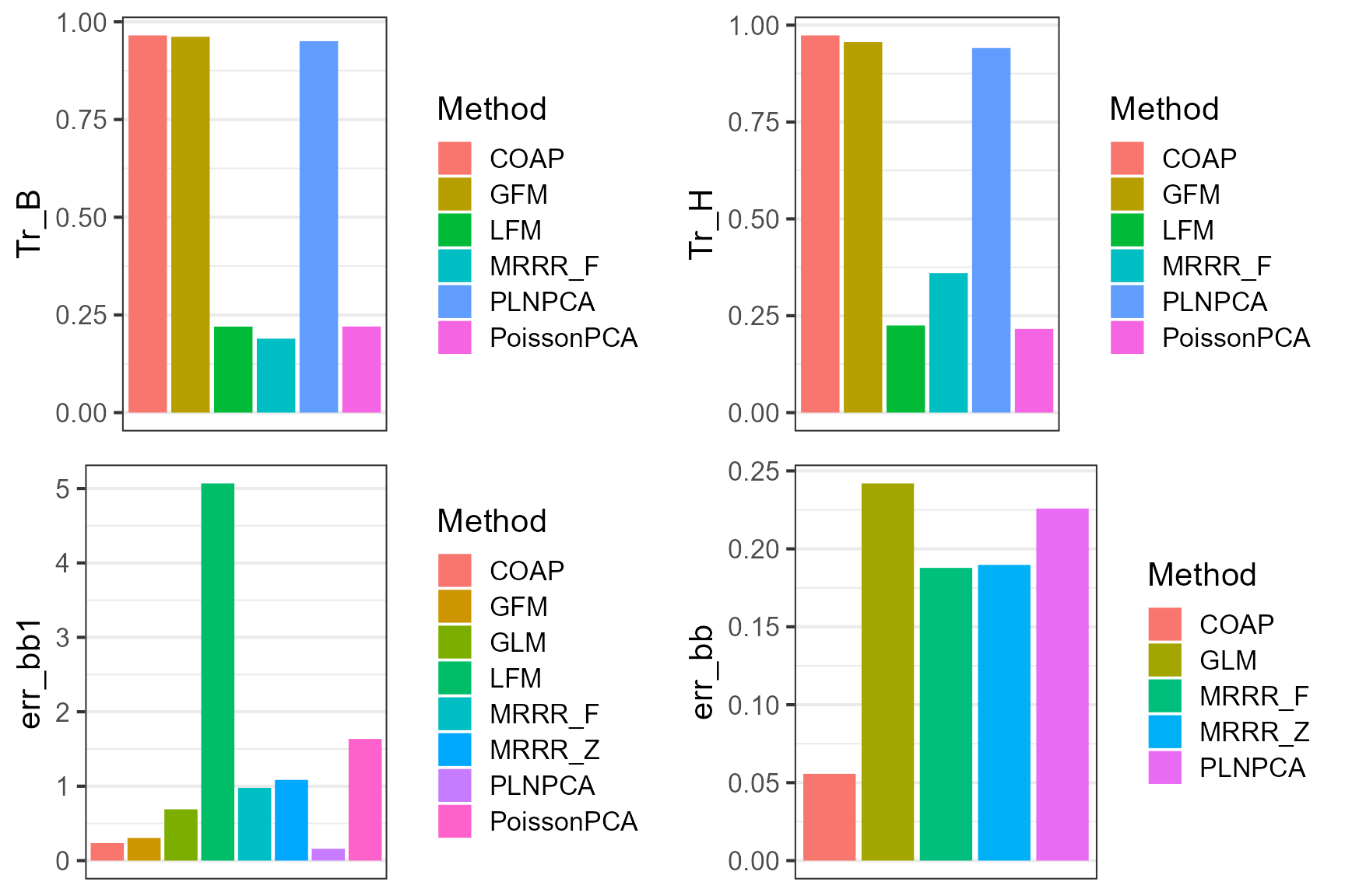
Select the parameters
We applied the singular value ratio based method to select the number of factors and the rank of coefficient matrix. The results showed that the SVR method has the potential to identify the true values.
datList <- gendata_simu(seed = 1, n=n, p=p, d= d, rank0 = rank0, q= q, rho=c(3, 6),
                        sigma2_eps = 1)
X_count <- datList$X; Z <- datList$Z
res1 <- selectParams(X_count=datList$X, Z=datList$Z, verbose=F)
#> Calculate initial values...

print(c(q_true=q, q_est=res1['hq']))
#>   q_true q_est.hq
#>        5        5
print(c(r_true=rank0, r_est=res1['hr']))
#>   r_true r_est.hr
#>        6        6
Session Info
sessionInfo()
#> R version 4.1.2 (2021-11-01)
#> Platform: x86_64-w64-mingw32/x64 (64-bit)
#> Running under: Windows 10 x64 (build 22621)
#>
#> Matrix products: default
#>
#> locale:
#> [1] LC_COLLATE=Chinese (Simplified)_China.936
#> [2] LC_CTYPE=Chinese (Simplified)_China.936
#> [3] LC_MONETARY=Chinese (Simplified)_China.936
#> [4] LC_NUMERIC=C
#> [5] LC_TIME=Chinese (Simplified)_China.936
#>
#> attached base packages:
#> [1] parallel  stats     graphics  grDevices utils     datasets  methods
#> [8] base
#>
#> other attached packages:
#>  [1] cowplot_1.1.1    rrpack_0.1-11    PLNmodels_1.0.1  PoissonPCA_1.0.3
#>  [5] ggplot2_3.4.1    irlba_2.3.5      Matrix_1.4-0     MASS_7.3-55
#>  [9] GFM_1.2.1        doSNOW_1.0.20    snow_0.4-4       iterators_1.0.14
#> [13] foreach_1.5.2    COAP_1.1
#>
#> loaded via a namespace (and not attached):
#>  [1] tidyr_1.2.0           sass_0.4.1            splines_4.1.2
#>  [4] bit64_4.0.5           jsonlite_1.8.0        bslib_0.3.1
#>  [7] assertthat_0.2.1      highr_0.9             yaml_2.3.6
#> [10] corrplot_0.92         globals_0.15.0        pillar_1.9.0
#> [13] lattice_0.20-45       glue_1.6.2            torch_0.9.1
#> [16] digest_0.6.29         colorspace_2.1-0      htmltools_0.5.2
#> [19] pkgconfig_2.0.3       listenv_0.8.0         purrr_0.3.4
#> [22] scales_1.2.1          processx_3.5.2        tibble_3.2.1
#> [25] generics_0.1.2        farver_2.1.1          cachem_1.0.6
#> [28] withr_2.5.0           cli_3.2.0             survival_3.2-13
#> [31] magrittr_2.0.3        crayon_1.5.1          memoise_2.0.1
#> [34] evaluate_0.15         ps_1.6.0              fs_1.5.2
#> [37] fansi_1.0.4           future_1.26.1         parallelly_1.32.0
#> [40] textshaping_0.3.6     tools_4.1.2           lifecycle_1.0.3
#> [43] lassoshooting_0.1.5-1 stringr_1.4.0         glassoFast_1.0
#> [46] glmnet_4.1-3          munsell_0.5.0         callr_3.7.0
#> [49] compiler_4.1.2        pkgdown_2.0.6         jquerylib_0.1.4
#> [52] systemfonts_1.0.4     rlang_1.1.0           grid_4.1.2
#> [55] nloptr_2.0.0          rstudioapi_0.13       igraph_1.3.5
#> [58] labeling_0.4.2        rmarkdown_2.11        gtable_0.3.3
#> [61] codetools_0.2-18      DBI_1.1.2             R6_2.5.1
#> [64] gridExtra_2.3         knitr_1.37            dplyr_1.0.9
#> [67] fastmap_1.1.0         future.apply_1.9.0    bit_4.0.4
#> [70] utf8_1.2.3            rprojroot_2.0.3       ragg_1.2.2
#> [73] coro_1.0.3            shape_1.4.6           desc_1.4.0
#> [76] stringi_1.7.6         Rcpp_1.0.10           vctrs_0.6.1
#> [79] tidyselect_1.1.2      xfun_0.29