This vignette introduces the usage of MultiCOAP for the analysis of high-dimensional count data with additional high-dimensional covariates, by comparison with other methods.
The package can be loaded with the command, and define some metric functions:
library(MultiCOAP)
#> Loading required package: irlba
#> Loading required package: Matrix
library(GFM)
#> Loading required package: doSNOW
#> Loading required package: foreach
#> Loading required package: iterators
#> Loading required package: snow
#> Loading required package: parallel
#>
#> Attaching package: 'parallel'
#> The following objects are masked from 'package:snow':
#>
#>     closeNode, clusterApply, clusterApplyLB, clusterCall, clusterEvalQ,
#>     clusterExport, clusterMap, clusterSplit, makeCluster, parApply,
#>     parCapply, parLapply, parRapply, parSapply, recvData, recvOneData,
#>     sendData, splitIndices, stopCluster
#> GFM :  Generalized factor model is implemented for ultra-high dimensional data with mixed-type variables.
#> Two algorithms, variational EM and alternate maximization, are designed to implement the generalized factor model,
#> respectively. The factor matrix and loading matrix together with the number of factors can be well estimated.
#> This model can be employed in social and behavioral sciences, economy and finance, and  genomics,
#> to extract interpretable nonlinear factors. More details can be referred to
#> Wei Liu, Huazhen Lin, Shurong Zheng and Jin Liu. (2021) <doi:10.1080/01621459.2021.1999818>.   Check out our Package website (https://feiyoung.github.io/GFM/docs/index.html) for a more complete description of the methods and analyses
normvec <- function(x) sqrt(sum(x^2)/ length(x))

trace_statistic_fun <- function(H, H0){

  tr_fun <- function(x) sum(diag(x))
  mat1 <- t(H0) %*% H %*% qr.solve(t(H) %*% H) %*% t(H) %*% H0

  tr_fun(mat1) / tr_fun(t(H0) %*% H0)

}
trace_list_fun <- function(Hlist, H0list){
  trvec <- rep(NA, length(Hlist))
  for(i in seq_along(trvec)){
    trvec[i] <- trace_statistic_fun(Hlist[[i]], H0list[[i]])
  }
  return(mean(trvec))
}
Generate the simulated data
First, we generate the data simulated data.
p <- 100; nvec <- c(200,300); d <- 10
methodNames <- c("MultiCOAP", "COAP", "MSFRlog", "MSFR")
metricMat <- matrix(NA, nrow=length(methodNames), ncol=6)
colnames(metricMat) <- c('A_tr', 'B_tr', 'beta_er', 'F_tr', 'H_tr', 'Time')
row.names(metricMat) <- methodNames

q <- 3; qs <- c(2,2); rank0 <- 2
rho<-c(2,3.5,0.1)
datList <- gendata_simu_multi2(seed = 1,nvec=nvec, p=p, d= d,
                                 q=q, qs=qs, rank0=rank0,rho=rho,sigma2_eps=1)
Fit the MultiCOAP model using the function MultiCOAP()
in the R package MultiCOAP. Users can use
?MultiCOAP to see the details about this function. For two
matrices
and
,
we use trace statistic to measure their similarity. The trace statistic
ranges from 0 to 1, with higher values indicating better performance. To
gauge the estimation accuracy of
,
we employ the mean estimation error (Er).
  XcList <- datList$Xlist;
  ZList <- datList$Zlist;
  res <- MultiCOAP(XcList, ZList, q=q, qs=qs,rank_use = rank0,init="MSFRVI")
#> iter = 2, ELBO= 2184343.536246, dELBO=1.001017
#> iter = 3, ELBO= 2192364.416467, dELBO=0.003672
#> iter = 4, ELBO= 2197355.147549, dELBO=0.002276
#> iter = 5, ELBO= 2196995.097790, dELBO=0.000164
#> iter = 6, ELBO= 2199809.993634, dELBO=0.001281
#> iter = 7, ELBO= 2201424.459731, dELBO=0.000734
#> iter = 8, ELBO= 2201999.929877, dELBO=0.000261
#> iter = 9, ELBO= 2202353.689072, dELBO=0.000161
#> iter = 10, ELBO= 2202610.919528, dELBO=0.000117
#> iter = 11, ELBO= 2202803.337119, dELBO=0.000087
#> iter = 12, ELBO= 2202946.216802, dELBO=0.000065
#> iter = 13, ELBO= 2203052.965942, dELBO=0.000048
#> iter = 14, ELBO= 2203135.021646, dELBO=0.000037
#> iter = 15, ELBO= 2203200.534665, dELBO=0.000030
#> iter = 16, ELBO= 2203254.477119, dELBO=0.000024
#> iter = 17, ELBO= 2203299.618271, dELBO=0.000020
#> iter = 18, ELBO= 2203337.582750, dELBO=0.000017
#> iter = 19, ELBO= 2203369.536121, dELBO=0.000015
#> iter = 20, ELBO= 2203396.463035, dELBO=0.000012
#> iter = 21, ELBO= 2203419.225522, dELBO=0.000010
#> iter = 22, ELBO= 2203438.560787, dELBO=0.000009
  #str(res)
  metricMat["MultiCOAP",'Time'] <- res$time.use
  metricMat["MultiCOAP",'A_tr'] <- trace_statistic_fun(res$A, datList$A0)
  metricMat["MultiCOAP",'B_tr'] <- trace_list_fun(res$B, datList$Blist0)
  metricMat["MultiCOAP",'F_tr'] <- trace_list_fun(res$F, datList$Flist)
  metricMat["MultiCOAP",'H_tr'] <- trace_list_fun(res$H, datList$Hlist)
  metricMat["MultiCOAP",'beta_er'] <- normvec(datList$bbeta0-res$bbeta)
Compare with other methods
We compare MultiCOAP with various prominent methods in the
literature. They are (1) covariate-augmented Possion factor model (COAP)
that disregards the study-specified factors and only estimates the
loadings and factors shared across studies, implemented in the R package
COAP; (2) newly developed multi-study factor regression
model (MSFR) with/without log(1+x) normalization for the observed count
data.
(1). First, we implemented covariate-augmented Possion factor model (COAP) and record the metrics that measure the estimation accuracy and computational cost.
mat2list <-function(z_int, nvec){

  zList_int <- list()
  istart <- 1
  for(i in 1:length(nvec)){

    zList_int[[i]] <- z_int[istart: sum(nvec[1:i]), ]
    istart <- istart + nvec[i]
  }
  return(zList_int)
}

COAP_run <- function(XcList, ZList, q, rank_use, aList=NULL, ...){

  require(COAP)
  nvec <- sapply(XcList, nrow)
  if(is.null(aList)){
    aList <- lapply(nvec, function(n1) rep(1, n1))
  }

  Xmat <- Reduce(rbind, XcList); Zmat <- Reduce( rbind, ZList)
  avec <- unlist(aList)
  tic <- proc.time()
  res_coap <- RR_COAP(Xmat, multiFac= avec, Z = Zmat,  q=q, rank_use=rank_use, ...)
  toc <- proc.time()
  res_coap$Flist <- mat2list(res_coap$H, nvec)
  res_coap$time.use <- toc[3] - tic[3]
  return(res_coap)
}

res_coap <- COAP_run(XcList, ZList, q=q,rank_use = rank0)
#> Loading required package: COAP
#> COAP :  A covariate-augmented overdispersed Poisson factor model is proposed to jointly perform a high-dimensional Poisson factor analysis and estimate a large coefficient matrix for overdispersed count data.
#> More details can be referred to Liu et al. (2024) <doi:10.1093/biomtc/ujae031>.
#> Calculate initial values...
#> iter = 2, ELBO= 2196208.907034, dELBO=1.001023
#> iter = 3, ELBO= 2200639.667769, dELBO=0.002017
#> iter = 4, ELBO= 2202502.097943, dELBO=0.000846
#> iter = 5, ELBO= 2203442.685804, dELBO=0.000427
#> iter = 6, ELBO= 2203974.249809, dELBO=0.000241
#> iter = 7, ELBO= 2204298.308810, dELBO=0.000147
#> iter = 8, ELBO= 2204506.620981, dELBO=0.000095
#> iter = 9, ELBO= 2204645.746279, dELBO=0.000063
#> iter = 10, ELBO= 2204741.378097, dELBO=0.000043
#> iter = 11, ELBO= 2204808.630051, dELBO=0.000031
#> iter = 12, ELBO= 2204856.826143, dELBO=0.000022
#> iter = 13, ELBO= 2204891.928375, dELBO=0.000016
#> iter = 14, ELBO= 2204917.856989, dELBO=0.000012
#> iter = 15, ELBO= 2204937.249320, dELBO=0.000009

metricMat["COAP",'Time']  <- res_coap$time.use
metricMat["COAP",'A_tr']  <- trace_statistic_fun(res_coap$B, datList$A0)
metricMat["COAP",'F_tr']  <- trace_list_fun(res_coap$Flist, datList$Flist)
metricMat["COAP",'beta_er']  <- normvec(datList$bbeta0-res_coap$bbeta)
(2). Then, we implemented multi-study factor regression model (MSFR) with/without log(1+x) normalization for the observed count data.
MSFR_run <- function(XcList, ZList, q, qs, maxIter=1e4, log.transform=FALSE, truncted=NULL, load.source=FALSE, dir.source=NULL){

  require(MSFA)
  require(psych)
  if(!load.source){
    source(paste0(dir.source, "MSFR_main_R_MSFR_V1.R"))
  }
  #fa <- psych::fa
  B_s <- ZList
  if(log.transform){
    X_s <- lapply(XcList, function(x) log(1+x))
  }else{
    X_s <- XcList #
  }
  if(!is.null(truncted)){
    replace_x <- function(x, truncted){
      x[x>truncted] <- truncted
      x[x<-truncted] <- -truncted
      return(x)
    }
    X_s <- lapply(X_s, replace_x, truncted=truncted)
  }
  t1<- proc.time()
  test <- start_msfa(X_s, B_s, 5, k=q, j_s=qs, constraint = "block_lower2", method = "adhoc")
  # EM_beta <- ecm_msfa(X_s, B_s, start=test, trace = FALSE, nIt=maxIter, constraint = "block_lower1")
  EM_beta <- ecm_msfa(X_s, B_s, start=test, trace = FALSE, nIt=maxIter)
  t2<- proc.time()
  EM_beta$Flist <- lapply(EM_beta$E_f, t)
  EM_beta$Hlist <- lapply(EM_beta$E_l, t)
  EM_beta$time.use <- t2[3] - t1[3]
  EM_beta$lambdavec <- sapply(EM_beta$psi_s,mean)
  return(EM_beta)
}
dir.source <- 'D:\\Working\\Research paper\\idea\\MultiPoisFactor\\Rpackage\\MultiCOAP\\simuCodes\\'

res_msfa <- MSFR_run(XcList, ZList, q=q, qs=qs, maxIter=1e3, log.transform=TRUE, dir.source = dir.source)
#> Loading required package: MSFA
#> Loading required package: psych
#> Loading required namespace: GPArotation
#> [1] 100
#> [1] 200
#> [1] 300
#> [1] 400
#> [1] 500
#> [1] 600
#> [1] 700
#> [1] 800
#> [1] 900
#> [1] 1000
metricMat["MSFRlog",'Time'] <- res_msfa$time.use
metricMat["MSFRlog",'A_tr'] <- trace_statistic_fun(res_msfa$Phi, datList$A0)
metricMat["MSFRlog",'B_tr']  <- trace_list_fun(res_msfa$Lambda_s, datList$Blist0)
metricMat["MSFRlog",'F_tr'] <- trace_list_fun(res_msfa$Flist, datList$Flist)
metricMat["MSFRlog",'H_tr'] <- trace_list_fun(res_msfa$Hlist, datList$Hlist)
metricMat["MSFRlog",'beta_er'] <- normvec(res_msfa$beta-datList$bbeta0)

res_msfa2 <- MSFR_run(XcList, ZList, q=q, qs=qs,truncted=500, maxIter=1e3, log.transform=FALSE, dir.source = dir.source)
#> [1] 100
#> [1] 200
#> [1] 300
#> [1] 400
#> [1] 500
#> [1] 600
#> [1] 700
#> [1] 800
#> [1] 900
#> [1] 1000
metricMat["MSFR",'Time'] <- res_msfa2$time.use
metricMat["MSFR",'A_tr'] <- trace_statistic_fun(res_msfa2$Phi, datList$A0)
metricMat["MSFR",'B_tr']  <- trace_list_fun(res_msfa2$Lambda_s, datList$Blist0)
metricMat["MSFR",'F_tr'] <- trace_list_fun(res_msfa2$Flist, datList$Flist)
metricMat["MSFR",'H_tr'] <- trace_list_fun(res_msfa2$Hlist, datList$Hlist)
metricMat["MSFR",'beta_er'] <- normvec(res_msfa2$beta-datList$bbeta0)
Visualize the comparison of performance
Next, we summarized the metrics for MultiCOAP and other compared methods in a data.frame object.
dat_metric <- data.frame(metricMat)
dat_metric$Method <- factor(row.names(dat_metric), levels=row.names(dat_metric))
Plot the results for MultiCOAP and other methods, which suggests that MultiCOAP achieves better estimation accuracy for the quantiites of interest.
library(cowplot)
library(ggplot2)
#>
#> Attaching package: 'ggplot2'
#> The following objects are masked from 'package:psych':
#>
#>     %+%, alpha
p1 <- ggplot(data=subset(dat_metric, !is.na(A_tr)), aes(x= Method, y=A_tr, fill=Method)) + geom_bar(stat="identity") + xlab(NULL) + scale_x_discrete(breaks=NULL) + theme_bw(base_size = 16)
p2 <- ggplot(data=subset(dat_metric, !is.na(F_tr)), aes(x= Method, y=F_tr, fill=Method)) + geom_bar(stat="identity") + xlab(NULL) + scale_x_discrete(breaks=NULL)+ theme_bw(base_size = 16)
p3 <- ggplot(data=subset(dat_metric, !is.na(B_tr)), aes(x= Method, y=B_tr, fill=Method)) + geom_bar(stat="identity") + xlab(NULL) + scale_x_discrete(breaks=NULL) + theme_bw(base_size = 16)
p4 <- ggplot(data=subset(dat_metric, !is.na(H_tr)), aes(x= Method, y=H_tr, fill=Method)) + geom_bar(stat="identity") + xlab(NULL) + scale_x_discrete(breaks=NULL)+ theme_bw(base_size = 16)
p5 <- ggplot(data=subset(dat_metric, !is.na(beta_er)), aes(x= Method, y=beta_er, fill=Method)) + geom_bar(stat="identity") + xlab(NULL) + scale_x_discrete(breaks=NULL)+ theme_bw(base_size = 16)
p6 <- ggplot(data=subset(dat_metric, !is.na(Time)), aes(x= Method, y=Time, fill=Method)) + geom_bar(stat="identity") + xlab(NULL) + scale_x_discrete(breaks=NULL)+ theme_bw(base_size = 16)
plot_grid(p1,p2,p3, p4, p5, p6, nrow=2, ncol=3)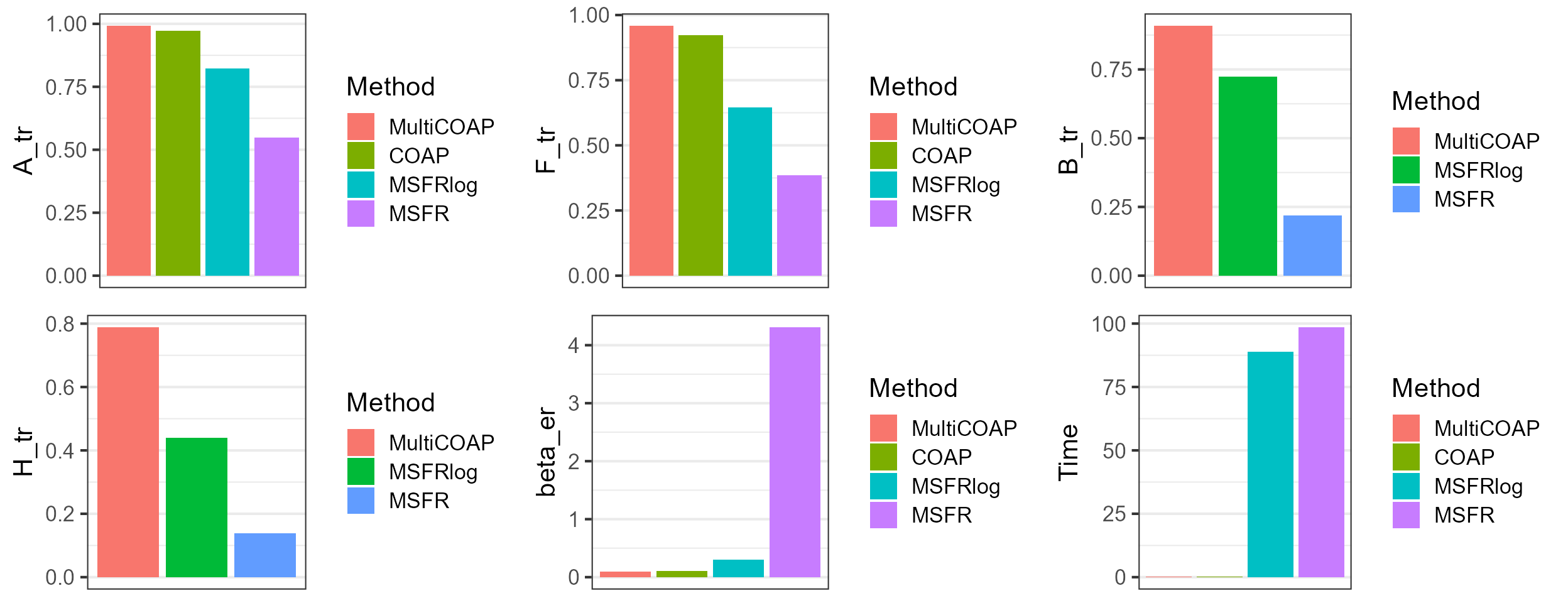
Select the parameters
We applied the proposed ‘CUP’ method to select the number of factors. The results showed that the CUP method has the potential to identify the true values.
selectQ <- function(res, tune.coef.rank=FALSE,  threshold=c(1e-1, 1e-2, 1e-2),
                    method=c("var.prop", "SVR"), upper.var.prop=0.95){

  method <- match.arg(method)
  qlist <- list()

  d_svdA <- svd(res$A)$d
  #
  if(method=='SVR'){
    d_svdA <- d_svdA[d_svdA>threshold[1]]
    qq <- length(d_svdA)
    if(qq>1){
      rsigs <- d_svdA[-qq]/d_svdA[-1]
      qlist$q <-  which.max(rsigs)
    }else{
      qlist$q <- 1
    }
  }else if(method=='var.prop'){
    prop.vec <- cumsum(d_svdA^2)/sum(d_svdA^2)
    qlist$q <- which(prop.vec> upper.var.prop)[1]
  }

  n_qs <- length(res$B)
  qvec <- rep(NA, n_qs)
  names(qvec) <- paste0("qs", 1:n_qs)
  for(i in 1:n_qs){
    # i <-1
    d_svdB1 <- svd(res$B[[i]])$d
    #
    if(method=='SVR'){
      d_svdB1 <- d_svdB1[d_svdB1>threshold[2]]
      qq1 <- length(d_svdB1)
      if(qq1>1){
        rsigB1 <- d_svdB1[-qq1]/d_svdB1[-1]
        qvec[i] <-  which.max(rsigB1)
      }else{
        qvec[i] <-  1
      }
    }else if(method=='var.prop'){
      prop.vec <- cumsum(d_svdB1^2)/sum(d_svdB1^2)
      qvec[i] <- which(prop.vec> upper.var.prop)[1]
    }
  }
  qlist$qs <- qvec
  return(qlist)
}

XcList <- datList$Xlist;
ZList <- datList$Zlist;
res <- MultiCOAP(XcList, ZList, q=q, qs=qs,rank_use = rank0,init="MSFRVI", verbose = FALSE)
hq.list <- selectQ(res, method='var.prop')
message("hq = ", hq.list$q, " VS true q = ", q)
#> hq = 3 VS true q = 3
message("hqs.vec = ", paste(hq.list$qs, collapse =", "), " VS true qs.vec = ", paste(qs, collapse =", "))
#> hqs.vec = 2, 2 VS true qs.vec = 2, 2
Session Info
sessionInfo()
#> R version 4.4.1 (2024-06-14 ucrt)
#> Platform: x86_64-w64-mingw32/x64
#> Running under: Windows 11 x64 (build 26100)
#>
#> Matrix products: default
#>
#>
#> locale:
#> [1] LC_COLLATE=Chinese (Simplified)_China.utf8
#> [2] LC_CTYPE=Chinese (Simplified)_China.utf8
#> [3] LC_MONETARY=Chinese (Simplified)_China.utf8
#> [4] LC_NUMERIC=C
#> [5] LC_TIME=Chinese (Simplified)_China.utf8
#>
#> time zone: Asia/Shanghai
#> tzcode source: internal
#>
#> attached base packages:
#> [1] parallel  stats     graphics  grDevices utils     datasets  methods
#> [8] base
#>
#> other attached packages:
#>  [1] ggplot2_3.5.1    cowplot_1.1.3    psych_2.4.6.26   MSFA_0.86
#>  [5] COAP_1.2         GFM_1.2.1        doSNOW_1.0.20    snow_0.4-4
#>  [9] iterators_1.0.14 foreach_1.5.2    MultiCOAP_1.1    irlba_2.3.5.1
#> [13] Matrix_1.7-0
#>
#> loaded via a namespace (and not attached):
#>  [1] gtable_0.3.5         xfun_0.47            bslib_0.8.0
#>  [4] htmlwidgets_1.6.4    lattice_0.22-6       vctrs_0.6.5
#>  [7] tools_4.4.1          generics_0.1.3       stats4_4.4.1
#> [10] tibble_3.2.1         fansi_1.0.6          highr_0.11
#> [13] DEoptimR_1.1-3       pkgconfig_2.0.3      desc_1.4.3
#> [16] lifecycle_1.0.4      farver_2.1.2         compiler_4.4.1
#> [19] GPArotation_2024.3-1 textshaping_0.4.0    statmod_1.5.0
#> [22] munsell_0.5.1        mnormt_2.1.1         codetools_0.2-20
#> [25] htmltools_0.5.8.1    sass_0.4.9           yaml_2.3.10
#> [28] pracma_2.4.4         pkgdown_2.1.1        pillar_1.9.0
#> [31] jquerylib_0.1.4      rrcov_1.7-6          MASS_7.3-60.2
#> [34] cachem_1.1.0         nlme_3.1-164         robustbase_0.99-4-1
#> [37] tidyselect_1.2.1     digest_0.6.37        mvtnorm_1.3-1
#> [40] dplyr_1.1.4          labeling_0.4.3       pcaPP_2.0-5
#> [43] robust_0.7-5         fastmap_1.2.0        grid_4.4.1
#> [46] colorspace_2.1-1     cli_3.6.3            magrittr_2.0.3
#> [49] utf8_1.2.4           withr_3.0.1          matlab_1.0.4.1
#> [52] scales_1.3.0         rmarkdown_2.28       ragg_1.3.3
#> [55] evaluate_1.0.0       knitr_1.48           rlang_1.1.4
#> [58] Rcpp_1.0.13          glue_1.7.0           fit.models_0.64
#> [61] rstudioapi_0.16.0    jsonlite_1.8.9       R6_2.5.1
#> [64] systemfonts_1.1.0    fs_1.6.4