High Dimensional Example of MultiRFM

This vignette introduces the usage of MultiRFM for the analysis of high-dimensional multi-study multivariate data with heavy tail, by comparison with other methods.

The package can be loaded with the command, and define some metric functions:

library(MultiRFM)
#> MultiRFM :  We introduce a high-dimensional multi-study robust factor model, called MultiRFM, which learns latent features and accounts for the heterogeneity among source. It could be used for analyzing heterogeneous RNA sequencing data. More details can be referred to Jiang et al. (2025) <doi:10.48550/arXiv.2506.18478>.
trace_statistic_fun <- function(H, H0){

  tr_fun <- function(x) sum(diag(x))
  mat1 <- t(H0) %*% H %*% qr.solve(t(H) %*% H) %*% t(H) %*% H0

  tr_fun(mat1) / tr_fun(t(H0) %*% H0)

}
trace_list_fun <- function(Hlist, H0list){
  trvec <- rep(NA, length(Hlist))
  for(i in seq_along(trvec)){
    trvec[i] <- trace_statistic_fun(Hlist[[i]], H0list[[i]])
  }
  return(mean(trvec))
}

Generate the simulated data

First, we generate the simulated data with heavy tail, where the error term follows from a multivariate t-distribution with degree of freedom 2.

nu <- 2 # nu is set to 
p <- 400
nvec <- c(150,200);  q <- 3;qs <- c(2,2); S <- length(nvec)
sigma2_eps <- 1
datList <- gendata_simu_multi(seed=1, nvec=nvec, p=p, q=q, qs=qs, rho=c(5,5), err.type='mvt', sigma2_eps = sigma2_eps, nu=nu)

Fit the MultiRFM model using the function MultiRFM() in the R package MultiRFM. Users can use ?MultiRFM to see the details about this function. For two matrices $\widehat D$ and $D$ , we use trace statistic to measure their similarity. The trace statistic ranges from 0 to 1, with higher values indicating better performance.

methodNames <- c("MultiRFM", "MSFA-CAVI", "MSFA-SVI")
metricMat <- matrix(NA, nrow=length(methodNames), ncol=5)
colnames(metricMat) <- c('A_tr', 'B_tr',  'F_tr', 'H_tr', 'Time')
row.names(metricMat) <- methodNames
XList <- datList$Xlist;

res <- MultiRFM(XList, q=q, qs=qs)
#> iter = 2, ELBO= -198771.450808, dELBO=0.999907 
#> iter = 3, ELBO= -186721.542969, dELBO=0.060622 
#> iter = 4, ELBO= -175550.044624, dELBO=0.059830 
#> iter = 5, ELBO= -173634.009351, dELBO=0.010914 
#> iter = 6, ELBO= -173079.027081, dELBO=0.003196 
#> iter = 7, ELBO= -172754.459964, dELBO=0.001875 
#> iter = 8, ELBO= -172511.815942, dELBO=0.001405 
#> iter = 9, ELBO= -172316.517503, dELBO=0.001132 
#> iter = 10, ELBO= -172154.416982, dELBO=0.000941 
#> iter = 11, ELBO= -172017.418560, dELBO=0.000796 
#> iter = 12, ELBO= -171900.109891, dELBO=0.000682 
#> iter = 13, ELBO= -171798.602463, dELBO=0.000591 
#> iter = 14, ELBO= -171709.990325, dELBO=0.000516 
#> iter = 15, ELBO= -171632.044887, dELBO=0.000454 
#> iter = 16, ELBO= -171563.023595, dELBO=0.000402 
#> iter = 17, ELBO= -171501.542405, dELBO=0.000358 
#> iter = 18, ELBO= -171446.487341, dELBO=0.000321 
#> iter = 19, ELBO= -171396.951399, dELBO=0.000289 
#> iter = 20, ELBO= -171352.188523, dELBO=0.000261 
#> iter = 21, ELBO= -171311.579431, dELBO=0.000237 
#> iter = 22, ELBO= -171274.605824, dELBO=0.000216 
#> iter = 23, ELBO= -171240.830673, dELBO=0.000197 
#> iter = 24, ELBO= -171209.882955, dELBO=0.000181 
#> iter = 25, ELBO= -171181.445704, dELBO=0.000166 
#> iter = 26, ELBO= -171155.246578, dELBO=0.000153 
#> iter = 27, ELBO= -171131.050319, dELBO=0.000141 
#> iter = 28, ELBO= -171108.652704, dELBO=0.000131 
#> iter = 29, ELBO= -171087.875630, dELBO=0.000121 
#> iter = 30, ELBO= -171068.563111, dELBO=0.000113
#str(res)
metricMat["MultiRFM",'Time'] <- res$time_use
metricMat["MultiRFM",'A_tr'] <- trace_statistic_fun(res$A, datList$A0)
metricMat["MultiRFM",'B_tr'] <- trace_list_fun(res$B, datList$Blist0)
metricMat["MultiRFM",'F_tr'] <- trace_list_fun(res$F, datList$Flist)
metricMat["MultiRFM",'H_tr'] <- trace_list_fun(res$H, datList$Hlist)

Compare with other methods

We compare MultiRFM with two prominent methods: MSFA-CAVI and MSFA-SVI

First, we implement MSFA-CAVI:

  X_s <- lapply(XList, scale, scale=FALSE)
  hmu <- sapply(XList, colMeans)
  library(VIMSFA)
  ### MSFA-CAVI
  print("MSFA-CAVI")
#> [1] "MSFA-CAVI"
  tic <- proc.time()
  cavi_est <- cavi_msfa(X_s,  K=q, J_s=qs)
#> [1] "Iteration:    1, Objective: 2.46722e+04, Relative improvement Inf"
#> [1] "Iteration:    1, Objective: 1.15704e+04, Relative improvement Inf"
#> [1] "Iteration:    1, Objective: 1.05719e+04, Relative improvement Inf"
#> [1] "Algorithm converged in 5 iterations."
  toc <- proc.time()
  time_cavi <- toc[3] - tic[3]
  hLam <- Reduce(cbind, cavi_est$mean_psi_s)
  hF_cavi <- hH_cavi <- list()
  for(s in 1:S){
    # s <- 1
    hF_cavi[[s]] <- t(Reduce(cbind, cavi_est$mean_f[[s]]))
    hH_cavi[[s]] <- t(Reduce(cbind, cavi_est$mean_l[[s]]))
  }
  
  metricMat["MSFA-CAVI",'Time']  <- time_cavi
  metricMat["MSFA-CAVI",'A_tr']  <- trace_statistic_fun(cavi_est$mean_phi, datList$A0)
  metricMat["MSFA-CAVI",'B_tr']  <- trace_list_fun(cavi_est$mean_lambda_s, datList$Blist0)
  metricMat["MSFA-CAVI",'F_tr'] <- trace_list_fun(hF_cavi, datList$Flist)
  metricMat["MSFA-CAVI",'H_tr'] <- trace_list_fun(hH_cavi, datList$Hlist)

Next, we implement MSFA-SVI:

  print("MSFA-SVI")
#> [1] "MSFA-SVI"
  tic <- proc.time()
  svi_est <- svi_msfa(X_s, K=q, J_s=qs, verbose = 0)
#> [1] "Iteration:    1, Objective: 2.44615e+04, Relative improvement Inf"
#> [1] "Iteration:    1, Objective: 1.15888e+04, Relative improvement Inf"
#> [1] "Iteration:    1, Objective: 1.05494e+04, Relative improvement Inf"
#> [1] "iteration 1 finished"
#> [1] "iteration 2 finished"
#> [1] "iteration 3 finished"
#> [1] "iteration 4 finished"
#> [1] "iteration 5 finished"
#> [1] "iteration 6 finished"
#> [1] "iteration 7 finished"
#> [1] "iteration 8 finished"
#> [1] "iteration 9 finished"
#> [1] "iteration 10 finished"
#> [1] "iteration 11 finished"
#> [1] "iteration 12 finished"
#> [1] "iteration 13 finished"
#> [1] "iteration 14 finished"
#> [1] "iteration 15 finished"
#> [1] "iteration 16 finished"
#> [1] "iteration 17 finished"
#> [1] "iteration 18 finished"
#> [1] "iteration 19 finished"
#> [1] "iteration 20 finished"
#> [1] "iteration 21 finished"
#> [1] "iteration 22 finished"
#> [1] "iteration 23 finished"
#> [1] "iteration 24 finished"
#> [1] "iteration 25 finished"
#> [1] "iteration 26 finished"
#> [1] "iteration 27 finished"
#> [1] "iteration 28 finished"
#> [1] "iteration 29 finished"
#> [1] "iteration 30 finished"
#> [1] "iteration 31 finished"
#> [1] "iteration 32 finished"
#> [1] "iteration 33 finished"
#> [1] "iteration 34 finished"
#> [1] "iteration 35 finished"
#> [1] "iteration 36 finished"
#> [1] "iteration 37 finished"
#> [1] "iteration 38 finished"
#> [1] "iteration 39 finished"
#> [1] "iteration 40 finished"
#> [1] "iteration 41 finished"
#> [1] "iteration 42 finished"
#> [1] "iteration 43 finished"
  toc <- proc.time()
  time_svi <- toc[3] - tic[3]
  hLam <- Reduce(cbind, svi_est$mean_psi_s)
  hF_cavi <- hH_cavi <- list()
  for(s in 1:S){
    # s <- 1
    hF_cavi[[s]] <- t(Reduce(cbind, svi_est$mean_f[[s]]))
    hH_cavi[[s]] <- t(Reduce(cbind, svi_est$mean_l[[s]]))
  }
  
  metricMat["MSFA-SVI",'Time']  <- time_cavi
  metricMat["MSFA-SVI",'A_tr']  <- trace_statistic_fun(svi_est$mean_phi, datList$A0)
  metricMat["MSFA-SVI",'B_tr']  <- trace_list_fun(svi_est$mean_lambda_s, datList$Blist0)
  metricMat["MSFA-SVI",'F_tr'] <- trace_list_fun(hF_cavi, datList$Flist)
  metricMat["MSFA-SVI",'H_tr'] <- trace_list_fun(hH_cavi, datList$Hlist)

Visualize the comparison of performance

Next, we summarized the metrics for MultiRFM and other compared methods in a data.frame object.



dat_metric <- data.frame(metricMat)
dat_metric$Method <- factor(row.names(dat_metric), levels=row.names(dat_metric))

Plot the results for MultiRFM and other methods, which suggests that MultiRFM achieves better estimation accuracy for the study-shared loading matrix A, study-specified loading matrix B and factor matrix H. MultiRFM significantly outperforms the compared methods in terms of estimation accuracy of B and H, as well as computational efficiency. The compared methods nearly failed to recover the study-specified loading and factor matrices.

library(cowplot)
library(ggplot2)
#> Warning: package 'ggplot2' was built under R version 4.4.3
p1 <- ggplot(data=subset(dat_metric, !is.na(A_tr)), aes(x= Method, y=A_tr, fill=Method)) + geom_bar(stat="identity") + xlab(NULL) + scale_x_discrete(breaks=NULL) + theme_bw(base_size = 16)
p2 <- ggplot(data=subset(dat_metric, !is.na(F_tr)), aes(x= Method, y=F_tr, fill=Method)) + geom_bar(stat="identity") + xlab(NULL) + scale_x_discrete(breaks=NULL)+ theme_bw(base_size = 16)
p3 <- ggplot(data=subset(dat_metric, !is.na(B_tr)), aes(x= Method, y=B_tr, fill=Method)) + geom_bar(stat="identity") + xlab(NULL) + scale_x_discrete(breaks=NULL) + theme_bw(base_size = 16)
p4 <- ggplot(data=subset(dat_metric, !is.na(H_tr)), aes(x= Method, y=H_tr, fill=Method)) + geom_bar(stat="identity") + xlab(NULL) + scale_x_discrete(breaks=NULL)+ theme_bw(base_size = 16)
p5 <- ggplot(data=subset(dat_metric, !is.na(Time)), aes(x= Method, y=Time, fill=Method)) + geom_bar(stat="identity") + xlab(NULL) + scale_x_discrete(breaks=NULL)+ theme_bw(base_size = 16)
plot_grid(p1,p2,p3, p4,  p5, nrow=2, ncol=3)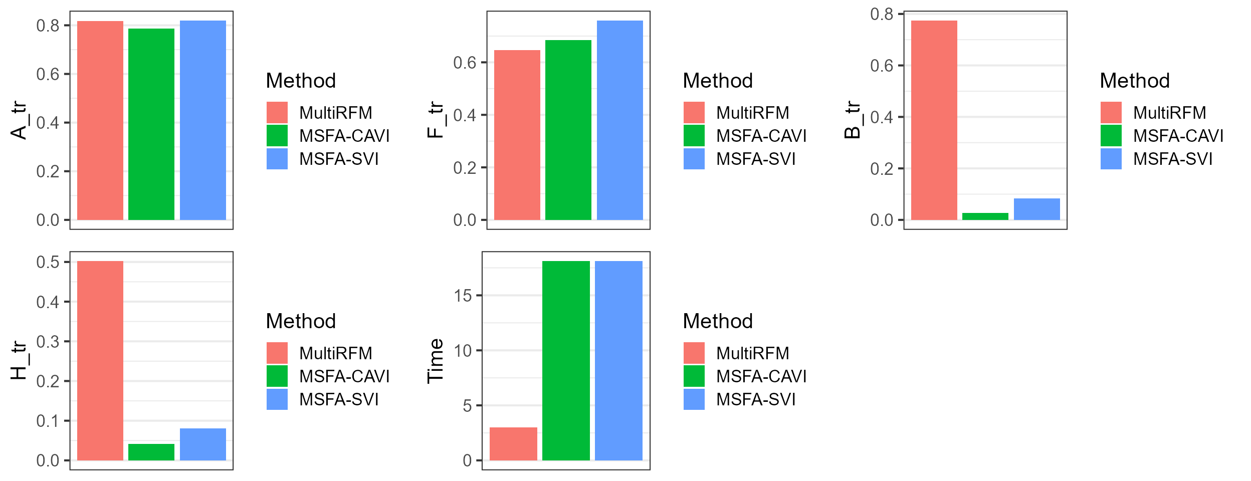

Select the parameters

We applied the proposed ‘CUP’ method to select the number of factors. The results showed that the CUP method has the potential to identify the true values.


datList <- gendata_simu_multi(seed=1, nvec=nvec, p=p, q=q, qs=qs, rho=c(5,5), err.type='mvt', sigma2_eps = 
                                sigma2_eps, nu=3)
XList <- datList$Xlist;
q_max <- 6; qs_max <- 4
hq.list <- selectFac.MultiRFM(XList,  q_max=q_max, qs_max=qs_max, verbose = FALSE)
message("hq = ", hq.list$q, " VS true q = ", q)
#> hq = 3 VS true q = 3
message("hqs.vec = ", paste(hq.list$qs, collapse =", "), " VS true qs.vec = ", paste(qs, collapse =", "))
#> hqs.vec = 2, 2 VS true qs.vec = 2, 2

Session Info

sessionInfo()
#> R version 4.4.1 (2024-06-14 ucrt)
#> Platform: x86_64-w64-mingw32/x64
#> Running under: Windows 11 x64 (build 26100)
#> 
#> Matrix products: default
#> 
#> 
#> locale:
#> [1] LC_COLLATE=Chinese (Simplified)_China.utf8 
#> [2] LC_CTYPE=Chinese (Simplified)_China.utf8   
#> [3] LC_MONETARY=Chinese (Simplified)_China.utf8
#> [4] LC_NUMERIC=C                               
#> [5] LC_TIME=Chinese (Simplified)_China.utf8    
#> 
#> time zone: Asia/Shanghai
#> tzcode source: internal
#> 
#> attached base packages:
#> [1] stats     graphics  grDevices utils     datasets  methods   base     
#> 
#> other attached packages:
#> [1] ggplot2_3.5.2  cowplot_1.1.3  VIMSFA_0.1.0   MultiRFM_1.1.0
#> 
#> loaded via a namespace (and not attached):
#>  [1] gtable_0.3.5         xfun_0.47            bslib_0.8.0         
#>  [4] htmlwidgets_1.6.4    lattice_0.22-6       vctrs_0.6.5         
#>  [7] tools_4.4.1          generics_0.1.3       parallel_4.4.1      
#> [10] tibble_3.2.1         fansi_1.0.6          highr_0.11          
#> [13] pkgconfig_2.0.3      Matrix_1.7-0         data.table_1.16.0   
#> [16] desc_1.4.3           lifecycle_1.0.4      compiler_4.4.1      
#> [19] farver_2.1.2         mixtools_2.0.0       textshaping_0.4.0   
#> [22] munsell_0.5.1        mnormt_2.1.1         htmltools_0.5.8.1   
#> [25] sass_0.4.9           yaml_2.3.10          lazyeval_0.2.2      
#> [28] plotly_4.10.4        pillar_1.9.0         pkgdown_2.1.1       
#> [31] jquerylib_0.1.4      tidyr_1.3.1          MASS_7.3-60.2       
#> [34] cachem_1.1.0         nlme_3.1-164         sparsepca_0.1.2     
#> [37] tidyselect_1.2.1     rsvd_1.0.5           digest_0.6.37       
#> [40] mvtnorm_1.3-1        dplyr_1.1.4          LaplacesDemon_16.1.6
#> [43] purrr_1.0.2          kernlab_0.9-33       labeling_0.4.3      
#> [46] splines_4.4.1        fastmap_1.2.0        grid_4.4.1          
#> [49] colorspace_2.1-1     cli_3.6.3            magrittr_2.0.3      
#> [52] survival_3.6-4       utf8_1.2.4           withr_3.0.1         
#> [55] scales_1.3.0         segmented_2.1-2      rmarkdown_2.28      
#> [58] httr_1.4.7           ragg_1.3.3           evaluate_1.0.0      
#> [61] knitr_1.48           irlba_2.3.5.1        viridisLite_0.4.2   
#> [64] rlang_1.1.4          Rcpp_1.0.13          glue_1.7.0          
#> [67] rstudioapi_0.16.0    jsonlite_1.8.9       R6_2.5.1            
#> [70] systemfonts_1.1.0    fs_1.6.4

Wei Liu

2025-11-26

Generate the simulated data

Compare with other methods

Visualize the comparison of performance

Select the parameters