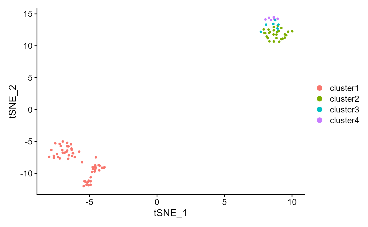
tNSE or UMAP plot visualization

Intuitive way of visualizing how cell types changes across the embeddings obatined by DR-SC.

drscPlot(seu, dims=1:5, visu.method='tSNE',...)

Arguments

seu

an object of class "Seurat" obtained by DR.SC.

dims

a positive integer to specify the number of latent features for visualiztion.

visu.method

a string including 'tSNE' or "UMAP".

...

Other arguments passing to DimPlot function.

Details

Nothing

Value

return a ggplot2 object.

References

None

Author

Wei Liu

Note

nothing

See also

None

Examples

## we generate the spatial transcriptomics data with lattice neighborhood, i.e. ST platform.
seu <- gendata_RNAExp(height=10, width=10,p=50, K=4)
library(Seurat)
seu <- NormalizeData(seu)
# choose spatially variable features
seu <- FindSVGs(seu)
#> Find the spatially variables genes by SPARK-X...
#> ## ===== SPARK-X INPUT INFORMATION ====
#> ## number of total samples: 100
#> ## number of total genes: 50
#> ## Running with single core, may take some time 
#> ## Testing With Projection Kernel
#> ## Testing With Gaussian Kernel 1
#> ## Testing With Gaussian Kernel 2
#> ## Testing With Gaussian Kernel 3
#> ## Testing With Gaussian Kernel 4
#> ## Testing With Gaussian Kernel 5
#> ## Testing With Cosine Kernel 1
#> ## Testing With Cosine Kernel 2
#> ## Testing With Cosine Kernel 3
#> ## Testing With Cosine Kernel 4
#> ## Testing With Cosine Kernel 5

# use SVGs to fit DR.SC model
# maxIter = 2 is only used for illustration, and user can use default.
seu1 <- DR.SC(seu, K=4,platform = 'ST', maxIter = 2,verbose=FALSE)
#> Neighbors were identified for 100 out of 100 spots.
#> Fit DR-SC model...
#> Using accurate PCA to obtain initial values
#> Finish DR-SC model fitting
drscPlot(seu1)