Generate the simulated data
First, we analyze a simulated spatial transcriptomics data from ST
platform, which is a Seurat object format. It is noted that the
meta.data must include spatial coordinates in columns named
“row” (x coordinates) and “col” (y coordinates)! This data is available
here.
load('sim_seu.rds')
library(DR.SC)
#> Loading required package: parallel
#> Loading required package: spatstat.geom
#> Loading required package: spatstat.data
#> Loading required package: spatstat.univar
#> spatstat.univar 3.0-1
#> spatstat.geom 3.3-3
#> DR.SC :  Joint dimension reduction and spatial clustering is conducted for
#> Single-cell RNA sequencing and spatial transcriptomics data, and more details can be referred to
#> Wei Liu, Xu Liao, Yi Yang, Huazhen Lin, Joe Yeong, Xiang Zhou, Xingjie Shi and Jin Liu. (2022) <doi:10.1093/nar/gkac219>. It is not only computationally efficient and scalable to the sample size increment, but also is capable of choosing the smoothness parameter and the number of clusters as well.   Check out our Package website (https://feiyoung.github.io/DR.SC/index.html) for a more complete description of the methods and analyses
head(seu@meta.data)
#>          orig.ident nCount_RNA nFeature_RNA row col imagerow imagecol
#> spot1 SeuratProject    1173170          500   1   1        1        1
#> spot2 SeuratProject    1526377          500   2   1        2        1
#> spot3 SeuratProject    1379906          500   3   1        3        1
#> spot4 SeuratProject    2603880          500   4   1        4        1
#> spot5 SeuratProject    2456589          500   5   1        5        1
#> spot6 SeuratProject    3331378          500   6   1        6        1
#>       true_clusters
#> spot1             1
#> spot2             1
#> spot3             1
#> spot4             4
#> spot5             4
#> spot6             4
Fit DR-SC using simulated data
Data preprocessing
This preprocessing includes Log-normalization and feature selection. Here we select highly variable genes for example first. The selected genes’ names are saved in “seu@assays$RNA@var.features”
### Given K
library(Seurat)
#> Loading required package: SeuratObject
#> Loading required package: sp
#>
#> Attaching package: 'SeuratObject'
#> The following objects are masked from 'package:base':
#>
#>     intersect, t
seu <- NormalizeData(seu)
#> Normalizing layer: counts
# choose highly variable features using Seurat
seu <- FindVariableFeatures(seu, nfeatures = 400)
#> Finding variable features for layer counts
Fit DR-SC based on highly variable genes(HVGs)
For function DR.SC, users can specify the number of
clusters
or set K to be an integer vector by using modified
BIC(MBIC) to determine
.
First, we try using user-specified number of clusters. Then we show the
version chosen by MBIC.
### Given K
seu2 <- DR.SC(seu, q=15, K=4, platform = 'ST',  verbose=F, approxPCA=T)
#> Neighbors were identified for 900 out of 900 spots.
#> Fit DR-SC model...
#> Using approxmated PCA to obtain initial values
#> Finish DR-SC model fitting
After finishing model fitting, we use ajusted rand index
(ARI) to check the performance of clustering
mclust::adjustedRandIndex(seu2$spatial.drsc.cluster, seu$true_clusters)
#> [1] 0.9914878
Next, we show the application of DR-SC in visualization. First, we can visualize the clusters from DR-SC on the spatial coordinates.
spatialPlotClusters(seu2)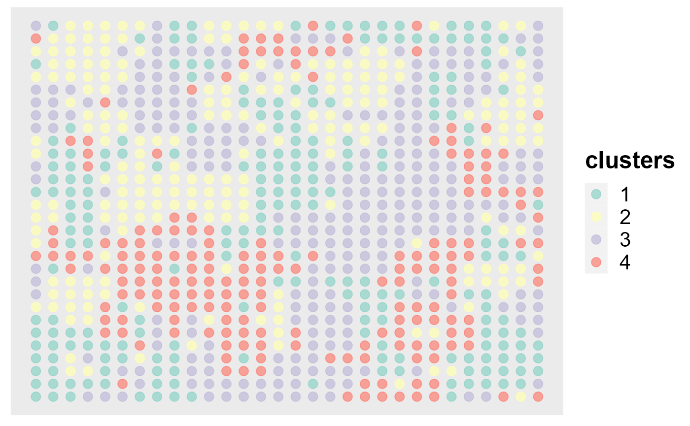
We can also visualize the clusters from DR-SC on the two-dimensional tSNE based on the extracted features from DR-SC.
drscPlot(seu2)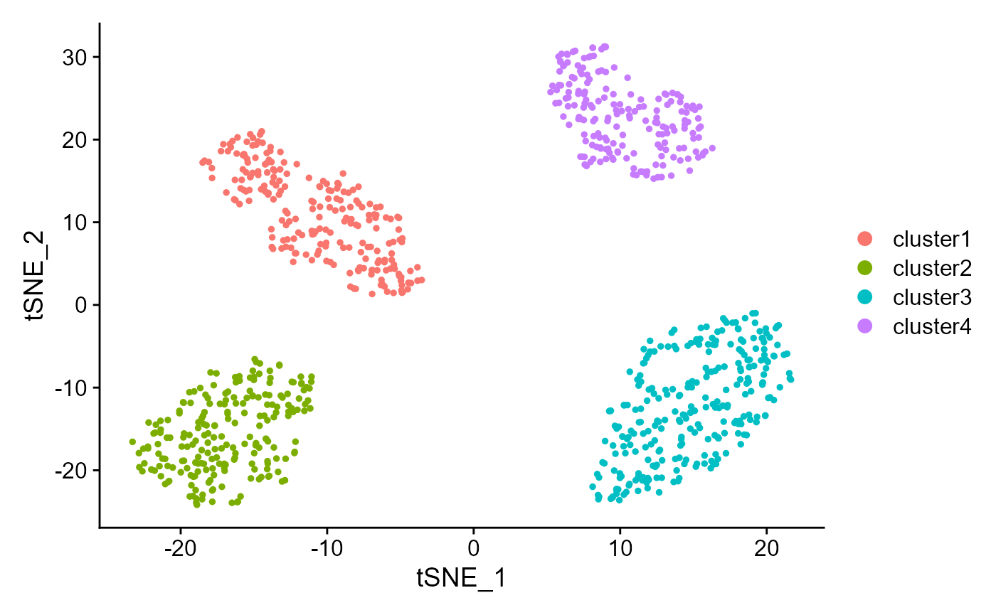 Show the UMAP plot based on the extracted features from DR-SC.
drscPlot(seu2, visu.method = 'UMAP')
#> Warning: The default method for RunUMAP has changed from calling Python UMAP via reticulate to the R-native UWOT using the cosine metric
#> To use Python UMAP via reticulate, set umap.method to 'umap-learn' and metric to 'correlation'
#> This message will be shown once per session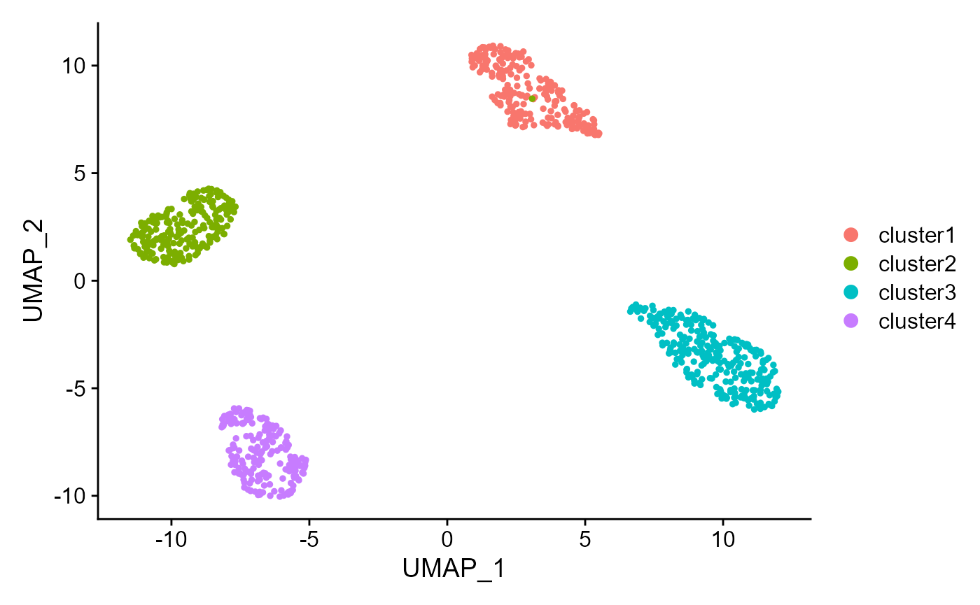
Use MBIC to choose number of clusters:
seu2 <- DR.SC(seu, q=10, K=2:6, platform = 'ST', verbose=F,approxPCA=T)
#> Neighbors were identified for 900 out of 900 spots.
#> Fit DR-SC model...
#> Using approxmated PCA to obtain initial values
#> Starting parallel computing intial values...
#> Finish DR-SC model fitting
mbicPlot(seu2)
Fit DR-SC based on spatially variable genes(SVGs)
First, we select the spatilly variable genes using funciton
FindSVGs.
### Given K
seu <- NormalizeData(seu, verbose=F)
# choose 400 spatially variable features using FindSVGs
seus <- FindSVGs(seu, nfeatures = 400, verbose = F)
seu2 <- DR.SC(seus, q=15, K=4, platform = 'ST', verbose=F)
#> Neighbors were identified for 900 out of 900 spots.
#> Fit DR-SC model...
#> Using accurate PCA to obtain initial values
#> Finish DR-SC model fitting
Using ARI to check the performance of clustering
mclust::adjustedRandIndex(seu2$spatial.drsc.cluster, seu$true_clusters)
#> [1] 0.9971493
DR-SC can enhance visualization
Show the spatial scatter plot for clusters
spatialPlotClusters(seu2)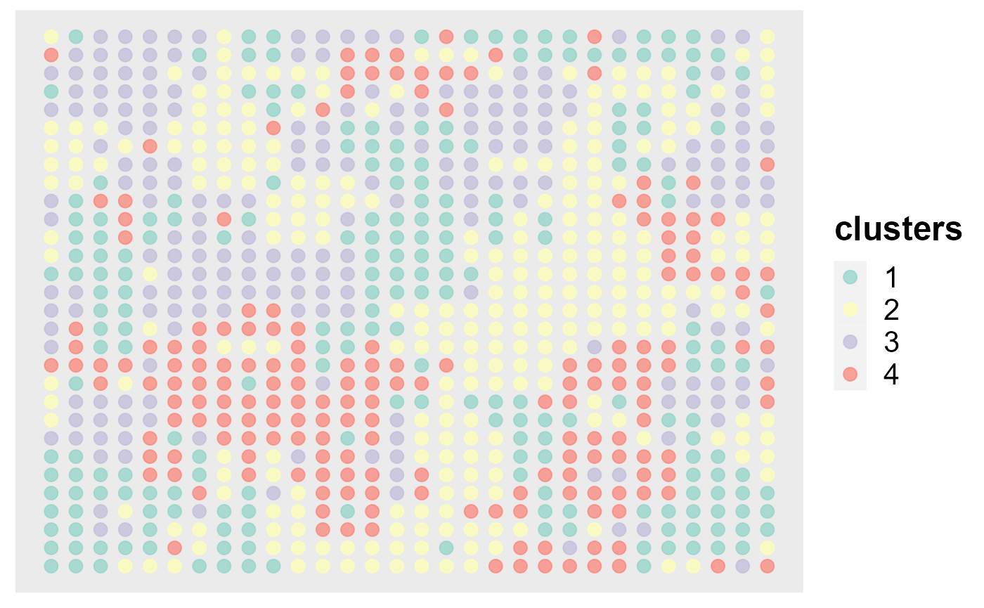
Show the tSNE plot based on the extracted features from DR-SC.
drscPlot(seu2)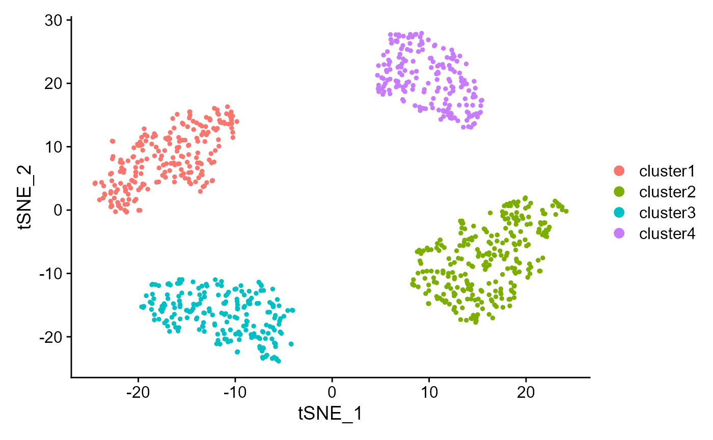 Show the UMAP plot based on the extracted features from DR-SC.
drscPlot(seu2, visu.method = 'UMAP')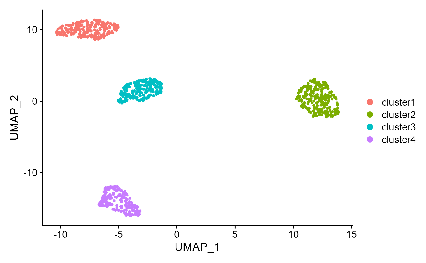
DR-SC can automatically determine the number of clusters
Use MBIC to choose number of clusters:
seu2 <- DR.SC(seus, q=4, K=2:6, platform = 'ST',  verbose=F)
#> Neighbors were identified for 900 out of 900 spots.
#> Fit DR-SC model...
#> Using accurate PCA to obtain initial values
#> Starting parallel computing intial values...
#> Finish DR-SC model fitting
mbicPlot(seu2)
# or plot BIC or AIC
# mbicPlot(seu2, criteria = 'BIC')
# mbicPlot(seu2, criteria = 'AIC')
# tune pen.const
seu2 <- selectModel(seu2, pen.const = 0.7)
mbicPlot(seu2)
DR-SC can help differentially expression analysis
Conduct visualization of marker gene expression. ### Ridge plots Visualize single cell expression distributions in each cluster from Seruat.
dat <- FindAllMarkers(seu2)
#> Calculating cluster cluster1
#> Calculating cluster cluster2
#> Calculating cluster cluster3
#> Calculating cluster cluster4
suppressPackageStartupMessages(library(dplyr) )
# Find the top 1 marker genes, user can change n to access more marker genes
dat %>%group_by(cluster) %>%
top_n(n = 1, wt = avg_log2FC) -> top
genes <- top$gene
RidgePlot(seu2, features = genes, ncol = 2)
#> Picking joint bandwidth of 0.131
#> Picking joint bandwidth of 0.136
#> Picking joint bandwidth of 0.117
#> Picking joint bandwidth of 0.235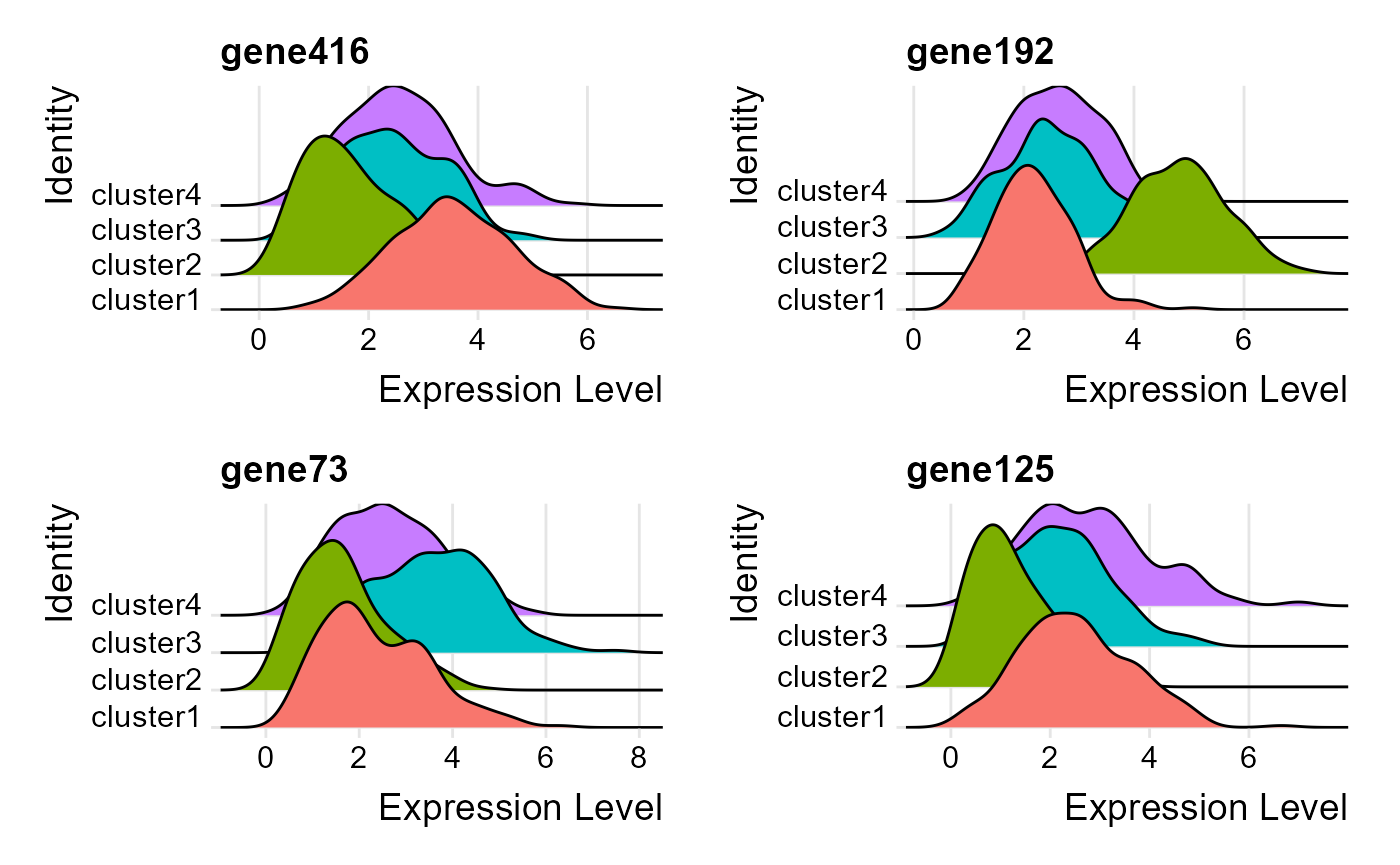 ### Violin plot Visualize single cell expression distributions in each
cluster
### Violin plot Visualize single cell expression distributions in each
cluster
VlnPlot(seu2, features = genes, ncol=2)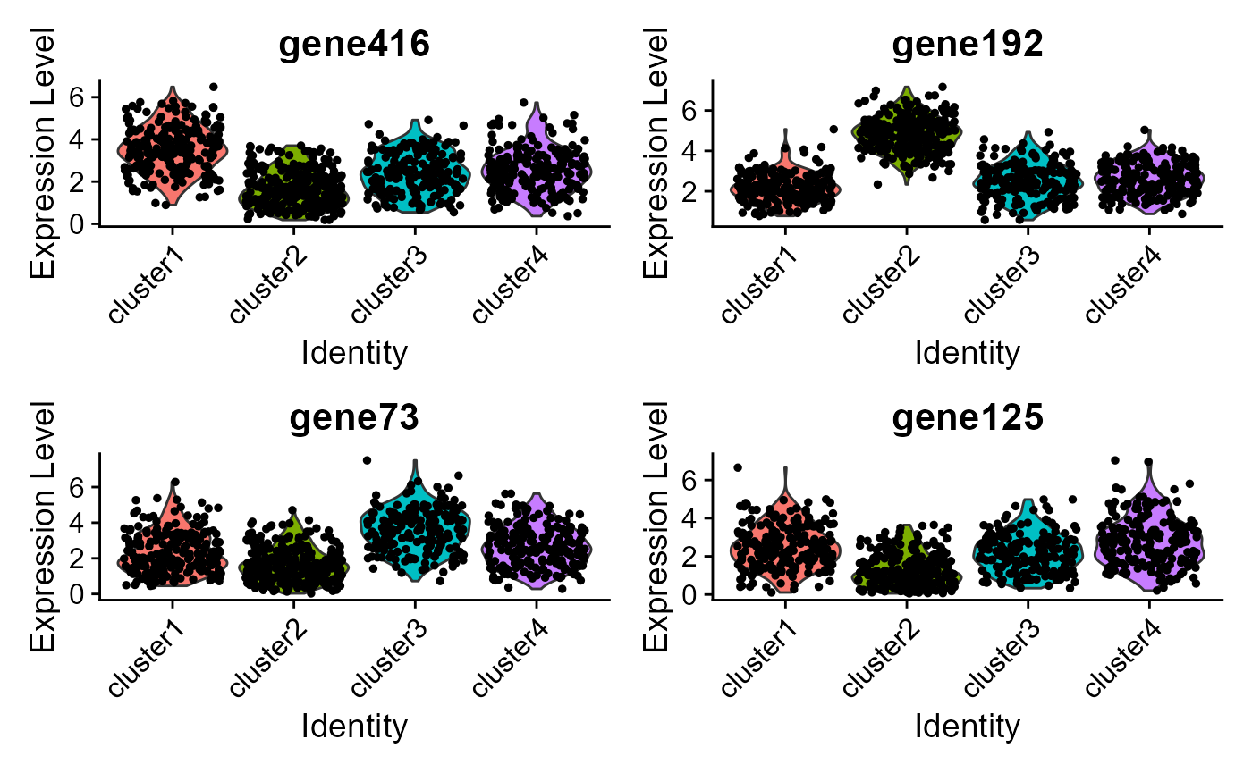 ### Feature plot We extract tSNE based on the features from DR-SC and
then visualize feature expression in the low-dimensional space
### Feature plot We extract tSNE based on the features from DR-SC and
then visualize feature expression in the low-dimensional space
seu2 <- RunTSNE(seu2, reduction="dr-sc", reduction.key='drsctSNE_')
#> Warning in `[[.DimReduc`(args$object, cells, args$dims): The following
#> embeddings are not present: NA
FeaturePlot(seu2, features = genes, reduction = 'tsne' ,ncol=2)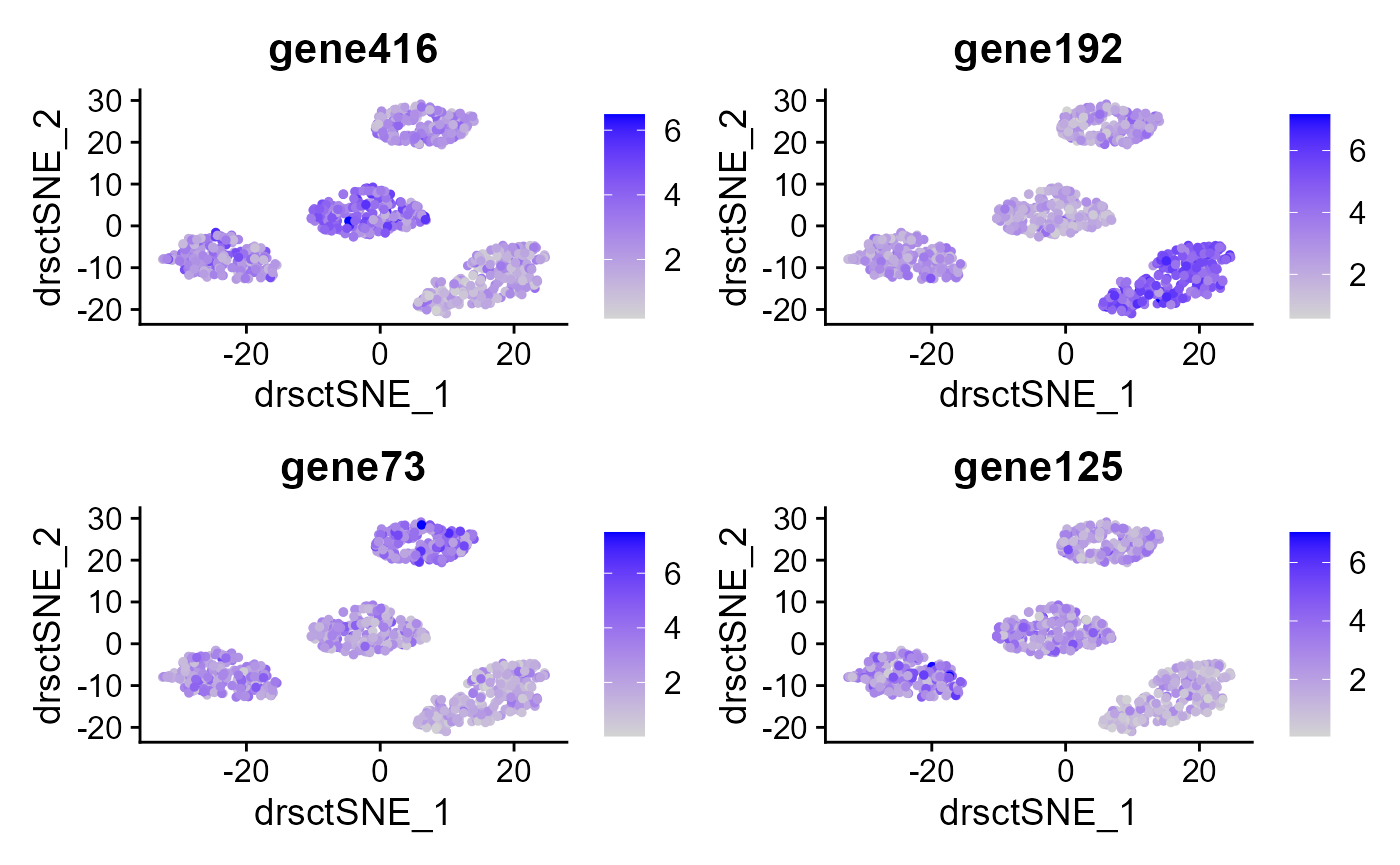
Dot plots
The size of the dot corresponds to the percentage of cells expressing the feature in each cluster. The color represents the average expression level
DotPlot(seu2, features = genes)
#> Warning: Scaling data with a low number of groups may produce misleading
#> results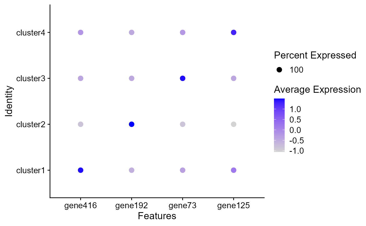
Heatmap plot
Single cell heatmap of feature expression
# standard scaling (no regression)
dat %>%group_by(cluster) %>%
    top_n(n = 30, wt = avg_log2FC) -> top
### select the marker genes that are also the variable genes.

genes <- intersect(top$gene, VariableFeatures(seu2))
## Change the HVGs to SVGs
#  <- topSVGs(seu2, 400)
seu2 <- ScaleData(seu2, verbose = F)
DoHeatmap(subset(seu2, downsample = 500),features = genes, size = 5)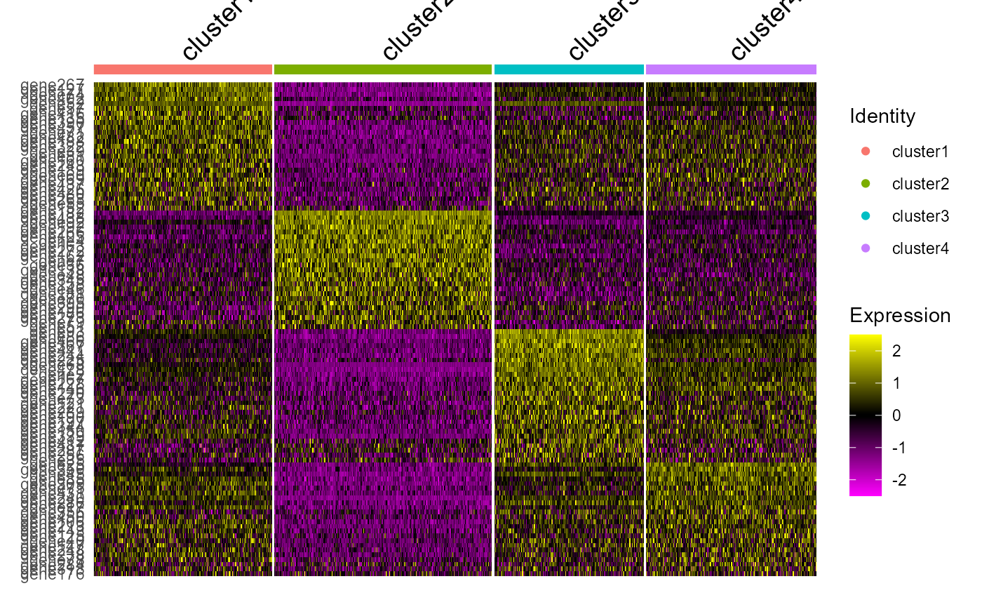
Session information
sessionInfo()
#> R version 4.4.1 (2024-06-14 ucrt)
#> Platform: x86_64-w64-mingw32/x64
#> Running under: Windows 11 x64 (build 26100)
#>
#> Matrix products: default
#>
#>
#> locale:
#> [1] LC_COLLATE=Chinese (Simplified)_China.utf8
#> [2] LC_CTYPE=Chinese (Simplified)_China.utf8
#> [3] LC_MONETARY=Chinese (Simplified)_China.utf8
#> [4] LC_NUMERIC=C
#> [5] LC_TIME=Chinese (Simplified)_China.utf8
#>
#> time zone: Asia/Shanghai
#> tzcode source: internal
#>
#> attached base packages:
#> [1] parallel  stats     graphics  grDevices utils     datasets  methods
#> [8] base
#>
#> other attached packages:
#> [1] dplyr_1.1.4           Seurat_5.1.0          SeuratObject_5.0.2
#> [4] sp_2.1-4              DR.SC_3.4             spatstat.geom_3.3-3
#> [7] spatstat.univar_3.0-1 spatstat.data_3.1-2
#>
#> loaded via a namespace (and not attached):
#>   [1] RColorBrewer_1.1-3     rstudioapi_0.16.0      jsonlite_1.8.9
#>   [4] magrittr_2.0.3         ggbeeswarm_0.7.2       spatstat.utils_3.1-0
#>   [7] farver_2.1.2           rmarkdown_2.28         fs_1.6.4
#>  [10] ragg_1.3.3             vctrs_0.6.5            ROCR_1.0-11
#>  [13] spatstat.explore_3.3-2 CompQuadForm_1.4.3     htmltools_0.5.8.1
#>  [16] sass_0.4.9             sctransform_0.4.1      parallelly_1.38.0
#>  [19] KernSmooth_2.23-24     bslib_0.8.0            htmlwidgets_1.6.4
#>  [22] desc_1.4.3             ica_1.0-3              plyr_1.8.9
#>  [25] plotly_4.10.4          zoo_1.8-12             cachem_1.1.0
#>  [28] igraph_2.0.3           mime_0.12              lifecycle_1.0.4
#>  [31] pkgconfig_2.0.3        Matrix_1.7-0           R6_2.5.1
#>  [34] fastmap_1.2.0          fitdistrplus_1.2-1     future_1.34.0
#>  [37] shiny_1.9.1            digest_0.6.37          colorspace_2.1-1
#>  [40] patchwork_1.3.0        S4Vectors_0.42.1       tensor_1.5
#>  [43] RSpectra_0.16-2        irlba_2.3.5.1          textshaping_0.4.0
#>  [46] labeling_0.4.3         progressr_0.14.0       fansi_1.0.6
#>  [49] spatstat.sparse_3.1-0  httr_1.4.7             polyclip_1.10-7
#>  [52] abind_1.4-8            compiler_4.4.1         withr_3.0.1
#>  [55] fastDummies_1.7.4      highr_0.11             MASS_7.3-60.2
#>  [58] tools_4.4.1            vipor_0.4.7            lmtest_0.9-40
#>  [61] beeswarm_0.4.0         httpuv_1.6.15          future.apply_1.11.2
#>  [64] goftest_1.2-3          glue_1.7.0             nlme_3.1-164
#>  [67] promises_1.3.0         grid_4.4.1             Rtsne_0.17
#>  [70] cluster_2.1.6          reshape2_1.4.4         generics_0.1.3
#>  [73] gtable_0.3.5           tidyr_1.3.1            data.table_1.16.0
#>  [76] utf8_1.2.4             BiocGenerics_0.50.0    RcppAnnoy_0.0.22
#>  [79] ggrepel_0.9.6          RANN_2.6.2             pillar_1.9.0
#>  [82] stringr_1.5.1          limma_3.58.1           spam_2.10-0
#>  [85] RcppHNSW_0.6.0         later_1.3.2            splines_4.4.1
#>  [88] lattice_0.22-6         survival_3.6-4         deldir_2.0-4
#>  [91] tidyselect_1.2.1       miniUI_0.1.1.1         pbapply_1.7-2
#>  [94] knitr_1.48             gridExtra_2.3          scattermore_1.2
#>  [97] stats4_4.4.1           xfun_0.47              statmod_1.5.0
#> [100] matrixStats_1.4.1      stringi_1.8.4          lazyeval_0.2.2
#> [103] yaml_2.3.10            evaluate_1.0.0         codetools_0.2-20
#> [106] tibble_3.2.1           cli_3.6.3              uwot_0.2.2
#> [109] xtable_1.8-4           reticulate_1.39.0      systemfonts_1.1.0
#> [112] munsell_0.5.1          jquerylib_0.1.4        Rcpp_1.0.13
#> [115] globals_0.16.3         spatstat.random_3.3-2  png_0.1-8
#> [118] ggrastr_1.0.2          pkgdown_2.1.1          ggplot2_3.5.2
#> [121] presto_1.0.0           dotCall64_1.1-1        mclust_6.1.1
#> [124] listenv_0.9.1          viridisLite_0.4.2      scales_1.3.0
#> [127] ggridges_0.5.6         leiden_0.4.3.1         purrr_1.0.2
#> [130] rlang_1.1.4            cowplot_1.1.3