The package can be loaded with the command:
set.seed(2024)
library("DR.SC")
#> Loading required package: parallel
#> Loading required package: spatstat.geom
#> Loading required package: spatstat.data
#> Loading required package: spatstat.univar
#> spatstat.univar 3.0-1
#> spatstat.geom 3.3-3
#> DR.SC :  Joint dimension reduction and spatial clustering is conducted for
#> Single-cell RNA sequencing and spatial transcriptomics data, and more details can be referred to
#> Wei Liu, Xu Liao, Yi Yang, Huazhen Lin, Joe Yeong, Xiang Zhou, Xingjie Shi and Jin Liu. (2022) <doi:10.1093/nar/gkac219>. It is not only computationally efficient and scalable to the sample size increment, but also is capable of choosing the smoothness parameter and the number of clusters as well.   Check out our Package website (https://feiyoung.github.io/DR.SC/index.html) for a more complete description of the methods and analyses
Fit DR-SC using real data DLPFC
To fit DR-SC model, we first require to create a Seurat object with meta.data including spatial coordinates in columns must named “row” (x coordinates) and “col” (y coordinates)!
Prepare Seurat object for DR-SC
We start this tutorial with creating the Seurat object. Users who are familar with Seurat object, can skip this subsection and go to next subsection.
First, we load the subset data of DLPFC 151510, dlpfc151510. Although it is saved as a Seurat object prepared for DR-SC, we re-create the Seurat object to show how to prepare the Seurat object for DR-SC.
data("dlpfc151510", package = 'DR.SC')Second, we create a Seurat object using the count matrix in dlpfc151510 and the spatial coordinates in the meta.data slot.
library(Seurat)
count <- dlpfc151510@assays$RNA@counts
meta_data <- data.frame(row=dlpfc151510@meta.data$row, col=dlpfc151510@meta.data$col, annotation=dlpfc151510$annotation)
row.names(meta_data) <- colnames(count)
## create Seurat object
dlpfc151510 <- CreateSeuratObject(counts=count, meta.data = meta_data)
head(dlpfc151510)
#>                       orig.ident nCount_RNA nFeature_RNA row col annotation
#> AAACAAGTATCTCCCA-1 SeuratProject        879          223  50 102     Layer1
#> AAACACCAATAACTGC-1 SeuratProject        887          251  59  19     Layer5
#> AAACAGAGCGACTCCT-1 SeuratProject       1109          253  14  94     Layer3
#> AAACAGCTTTCAGAAG-1 SeuratProject       1652          325  43   9     Layer4
#> AAACAGGGTCTATATT-1 SeuratProject       1389          289  47  13     Layer4
#> AAACAGTGTTCCTGGG-1 SeuratProject        758          226  73  43     Layer6
#> AAACATGGTGAGAGGA-1 SeuratProject        750          235  62   0         WM
#> AAACATTTCCCGGATT-1 SeuratProject       1946          332  61  97     Layer3
#> AAACCCGAACGAAATC-1 SeuratProject        798          244  45 115     Layer1
#> AAACCGGAAATGTTAA-1 SeuratProject        796          217  54 124     Layer2
Until now, the data preparation with Seurat object format is finished, and we can go to next step: preprocessing.
Data preprocessing
This preprocessing includes Log-normalization and feature selection. Here we select highly variable genes for example first. The selected genes’ names are saved in “VariableFeatures(seu)”.
# standard log-normalization
dlpfc151510 <- NormalizeData(dlpfc151510, verbose = F)
# choose 500 highly variable features
seu <- FindVariableFeatures(dlpfc151510, nfeatures = 500, verbose = F)
VariableFeatures(seu)[1:10]
#>  [1] "ENSG00000123560" "ENSG00000197971" "ENSG00000122585" "ENSG00000211592"
#>  [5] "ENSG00000244734" "ENSG00000110484" "ENSG00000091513" "ENSG00000109846"
#>  [9] "ENSG00000173786" "ENSG00000131095"
Fit DR-SC model using 500 highly variable features
We fit the DR-SC model by using the highly variable genes.
### Given K
seu <- DR.SC(seu, K=7, platform = 'Visium', verbose=T, approxPCA=T)
#> Neighbors were identified for 4634 out of 4634 spots.
#> Fit DR-SC model...
#> -------------------Calculate inital values-------------
#> Using approxmated PCA to obtain initial values
#> -------------------Finish computing inital values-------------
#> -------------------Starting  ICM-EM algortihm-------------
#> iter = 2, loglik= -1277658.515890, dloglik=0.999872
#> iter = 3, loglik= -1270070.341790, dloglik=0.005939
#> iter = 4, loglik= -1267934.809732, dloglik=0.001681
#> iter = 5, loglik= -1266820.486746, dloglik=0.000879
#> iter = 6, loglik= -1266053.381072, dloglik=0.000606
#> iter = 7, loglik= -1265467.376889, dloglik=0.000463
#> iter = 8, loglik= -1264981.092803, dloglik=0.000384
#> iter = 9, loglik= -1264565.826939, dloglik=0.000328
#> iter = 10, loglik= -1264214.650850, dloglik=0.000278
#> iter = 11, loglik= -1263911.158089, dloglik=0.000240
#> iter = 12, loglik= -1263644.542523, dloglik=0.000211
#> iter = 13, loglik= -1263418.343068, dloglik=0.000179
#> iter = 14, loglik= -1263218.529071, dloglik=0.000158
#> iter = 15, loglik= -1263034.248967, dloglik=0.000146
#> iter = 16, loglik= -1262871.138195, dloglik=0.000129
#> iter = 17, loglik= -1262718.922605, dloglik=0.000121
#> iter = 18, loglik= -1262588.514786, dloglik=0.000103
#> iter = 19, loglik= -1262467.080937, dloglik=0.000096
#> iter = 20, loglik= -1262349.032526, dloglik=0.000094
#> iter = 21, loglik= -1262244.078363, dloglik=0.000083
#> iter = 22, loglik= -1262142.961237, dloglik=0.000080
#> iter = 23, loglik= -1262051.580988, dloglik=0.000072
#> iter = 24, loglik= -1261972.339513, dloglik=0.000063
#> iter = 25, loglik= -1261894.196150, dloglik=0.000062
#> -------------------Complete!-------------
#> elasped time is :50.02
#> Finish DR-SC model fitting
Visualization
mclust::adjustedRandIndex(seu$spatial.drsc.cluster, seu$annotation)
#> [1] 0.509726
spatialPlotClusters(seu)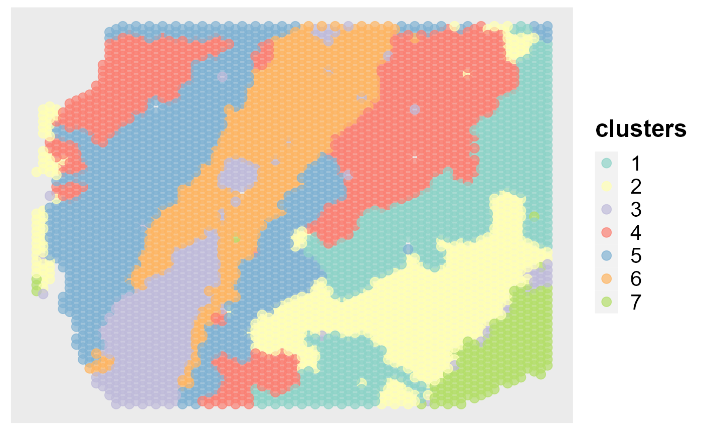
Show the tSNE plot based on the extracted features from DR-SC.
drscPlot(seu)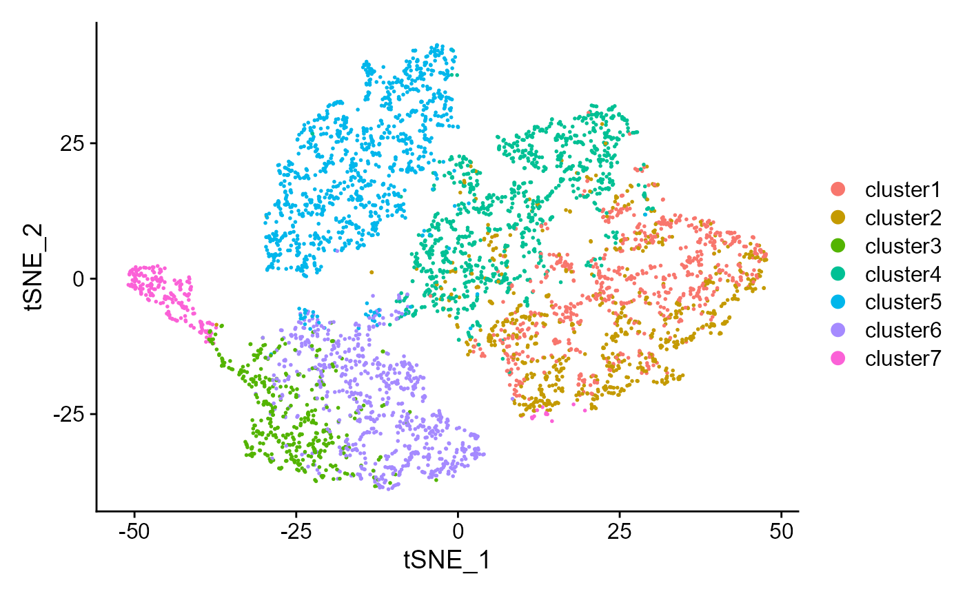
Show the UMAP plot based on the extracted features from DR-SC.
drscPlot(seu, visu.method = 'UMAP')
#> Warning: The default method for RunUMAP has changed from calling Python UMAP via reticulate to the R-native UWOT using the cosine metric
#> To use Python UMAP via reticulate, set umap.method to 'umap-learn' and metric to 'correlation'
#> This message will be shown once per session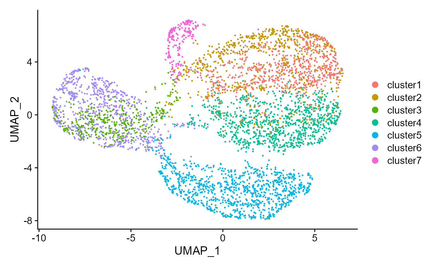
Fit DR-SC model using 480 spatially variable features
In spatially resolved transcriptomics data analysis, we recommend
users using the spatially variable genes for analysis. We embeded the
method SPARK-X (developed by Xiang Zhou’s Lab) into DR.SC package, which
can be called using FindSVGs. The selected genes’ names are
also saved in “seus@assays$RNA@var.features” and the order is determined by the
statistical significance, where the gene with highest significance ranks
first. We note there are some difference between SVGs and HVGs.
# choose 480 spatially variable features
seus <- FindSVGs(seu, nfeatures = 480)
#> Find the spatially variables genes by SPARK-X...
#> ## ===== SPARK-X INPUT INFORMATION ====
#> ## number of total samples: 4634
#> ## number of total genes: 500
#> ## Running with single core, may take some time
#> ## Testing With Projection Kernel
#> ## Testing With Gaussian Kernel 1
#> ## Testing With Gaussian Kernel 2
#> ## Testing With Gaussian Kernel 3
#> ## Testing With Gaussian Kernel 4
#> ## Testing With Gaussian Kernel 5
#> ## Testing With Cosine Kernel 1
#> ## Testing With Cosine Kernel 2
#> ## Testing With Cosine Kernel 3
#> ## Testing With Cosine Kernel 4
#> ## Testing With Cosine Kernel 5
VariableFeatures(seu)[1:10]
#>  [1] "ENSG00000123560" "ENSG00000197971" "ENSG00000122585" "ENSG00000211592"
#>  [5] "ENSG00000244734" "ENSG00000110484" "ENSG00000091513" "ENSG00000109846"
#>  [9] "ENSG00000173786" "ENSG00000131095"
We fit DR-SC model by using the selected spatially variable genes.
### Given K
seus <- DR.SC(seus,  K=7, platform = 'Visium', verbose=F, approxPCA=T)
#> Neighbors were identified for 4634 out of 4634 spots.
#> Fit DR-SC model...
#> Using approxmated PCA to obtain initial values
#> Finish DR-SC model fitting
Visualization
Next, we show the application of DR-SC in visualization. First, we can visualize the clusters from DR-SC on the spatial coordinates.
spatialPlotClusters(seus)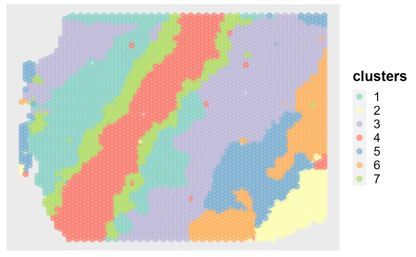
mclust::adjustedRandIndex(seus$spatial.drsc.cluster, seus$annotation)
#> [1] 0.4945463
We can also visualize the clusters from DR-SC on the two-dimensional tSNE based on the extracted features from DR-SC.
drscPlot(seus)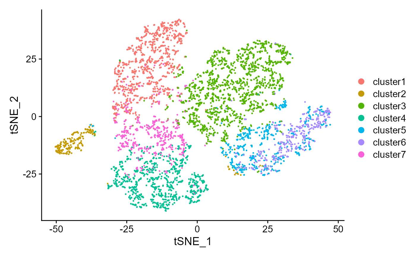 Similarly, can also visualize the clusters from DR-SC on the
two-dimensional UMAP based on the extracted features from DR-SC.
Similarly, can also visualize the clusters from DR-SC on the
two-dimensional UMAP based on the extracted features from DR-SC.
drscPlot(seus, visu.method = 'UMAP')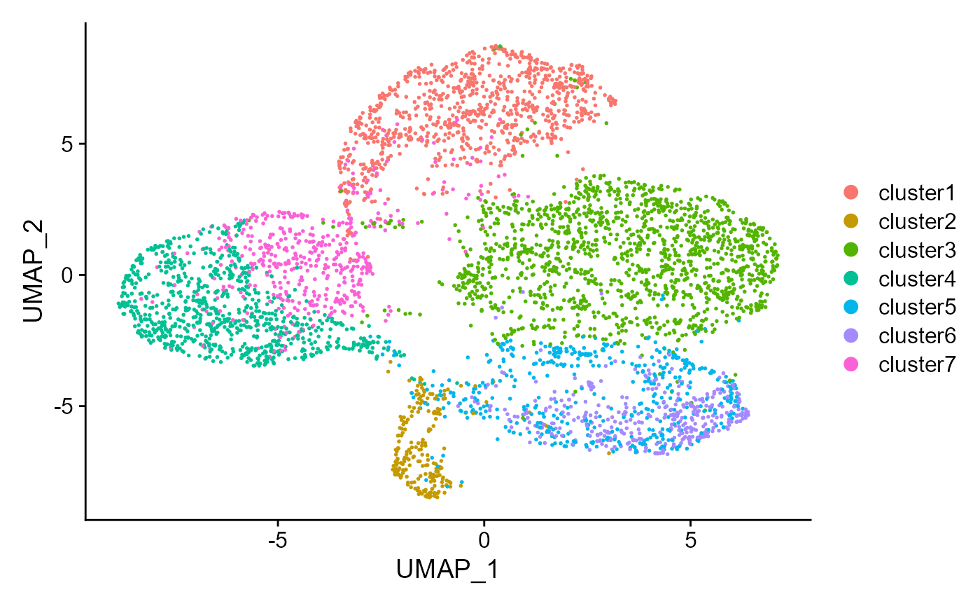
Since DR.SC uses the Seurat object to save results, all visualization functions in Seurat package can used to visualize the results of DR-SC, such as ridge plot, feature plot, dot plot and so on. ### Ridge plots we show the application of DR-SC in differential expression analysis. Find the marker genes in SVGs for each clusters.
SVGs <- topSVGs(seus, ntop = 400)
dat <- FindAllMarkers(seus, features = SVGs)
#> Calculating cluster cluster1
#> Calculating cluster cluster2
#> Calculating cluster cluster3
#> Calculating cluster cluster4
#> Calculating cluster cluster5
#> Calculating cluster cluster6
#> Calculating cluster cluster7
head(dat)
#>                        p_val avg_log2FC pct.1 pct.2    p_val_adj  cluster
#> ENSG00000131095 3.458652e-77  2.5527586 0.897 0.685 1.729326e-74 cluster1
#> ENSG00000251562 4.774071e-35  1.6717831 0.804 0.799 2.387036e-32 cluster1
#> ENSG00000198840 3.299012e-29 -0.4223879 0.958 1.000 1.649506e-26 cluster1
#> ENSG00000128656 1.015385e-24 -0.8879627 0.402 0.862 5.076926e-22 cluster1
#> ENSG00000154146 4.560970e-22 -0.6551079 0.682 0.949 2.280485e-19 cluster1
#> ENSG00000143013 1.034270e-21 -1.0654096 0.220 0.679 5.171349e-19 cluster1
#>                            gene
#> ENSG00000131095 ENSG00000131095
#> ENSG00000251562 ENSG00000251562
#> ENSG00000198840 ENSG00000198840
#> ENSG00000128656 ENSG00000128656
#> ENSG00000154146 ENSG00000154146
#> ENSG00000143013 ENSG00000143013
library(dplyr, verbose=F)
#>
#> Attaching package: 'dplyr'
#> The following objects are masked from 'package:stats':
#>
#>     filter, lag
#> The following objects are masked from 'package:base':
#>
#>     intersect, setdiff, setequal, union
top2 <-  dat %>%
  group_by(cluster) %>%
  top_n(n = 2, wt = avg_log2FC)
top2
#> # A tibble: 14 × 7
#> # Groups:   cluster [7]
#>        p_val avg_log2FC pct.1 pct.2 p_val_adj cluster  gene
#>        <dbl>      <dbl> <dbl> <dbl>     <dbl> <fct>    <chr>
#>  1 3.46e- 77       2.55 0.897 0.685 1.73e- 74 cluster1 ENSG00000131095
#>  2 2.16e- 12       1.99 0.453 0.346 1.08e-  9 cluster1 ENSG00000113140
#>  3 1.90e- 49       1.79 0.448 0.264 9.50e- 47 cluster2 ENSG00000171885
#>  4 5.60e- 44       1.58 0.47  0.309 2.80e- 41 cluster2 ENSG00000182600
#>  5 5.65e- 47       1.66 0.412 0.173 2.82e- 44 cluster3 ENSG00000183036
#>  6 1.07e- 30       1.53 0.236 0.082 5.37e- 28 cluster3 ENSG00000158258
#>  7 5.06e- 99       1.13 0.643 0.304 2.53e- 96 cluster4 ENSG00000104722
#>  8 1.89e- 40       1.11 0.267 0.107 9.43e- 38 cluster4 ENSG00000100285
#>  9 3.82e- 28       2.50 0.533 0.175 1.91e- 25 cluster5 ENSG00000168314
#> 10 4.43e- 16       2.68 0.346 0.113 2.21e- 13 cluster5 ENSG00000105695
#> 11 3.26e-142       1.33 0.756 0.379 1.63e-139 cluster6 ENSG00000115756
#> 12 1.04e- 25       1.10 0.233 0.114 5.20e- 23 cluster6 ENSG00000125869
#> 13 1.66e-147       4.38 1     0.164 8.32e-145 cluster7 ENSG00000168314
#> 14 3.87e-135       4.15 0.817 0.1   1.94e-132 cluster7 ENSG00000013297
Visualize single cell expression distributions in each cluster from Seruat.
genes <- top2$gene[seq(1, 12, by=2)]
RidgePlot(seus, features = genes, ncol = 2)
#> Picking joint bandwidth of 0.255
#> Picking joint bandwidth of 0.301
#> Picking joint bandwidth of 0.049
#> Picking joint bandwidth of 0.126
#> Picking joint bandwidth of 0.158
#> Picking joint bandwidth of 0.211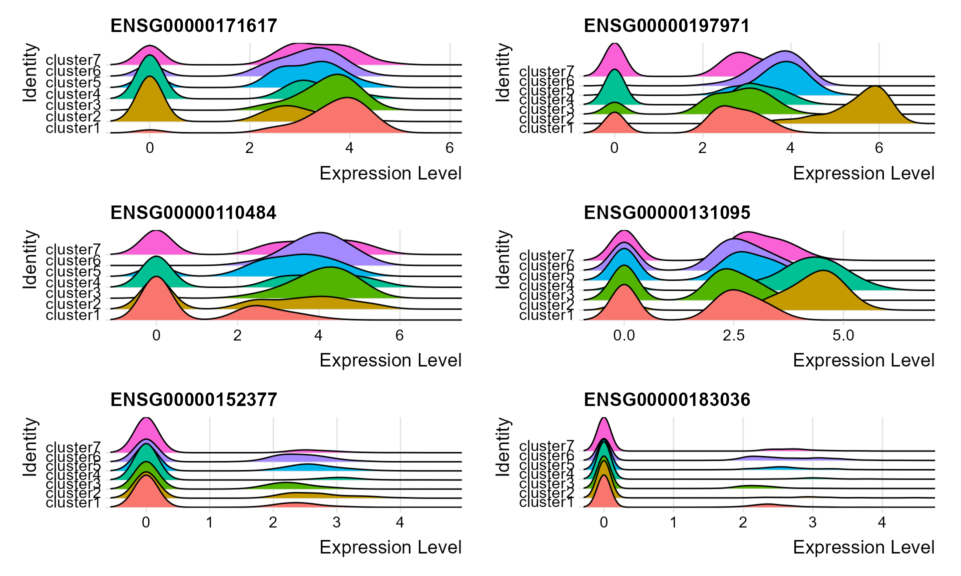 ### Violin plot
Visualize single cell expression distributions in each cluster
VlnPlot(seus, features = genes, ncol=2)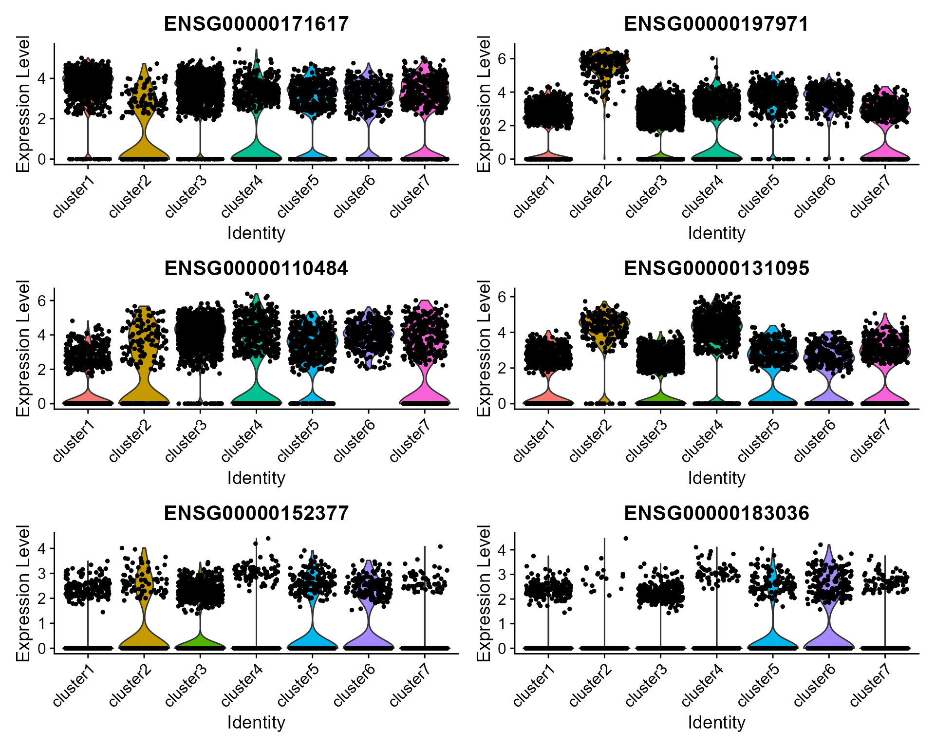
Feature plot
We extract tSNE based on the features from DR-SC and then visualize feature expression in the low-dimensional space
seus <- RunTSNE(seus, reduction="dr-sc", reduction.key='drsc_tSNE_')
#> Warning: Keys should be one or more alphanumeric characters followed by an
#> underscore, setting key from drsc_tSNE_ to drsctSNE_
FeaturePlot(seus, features = genes, reduction = 'tsne' ,ncol=2)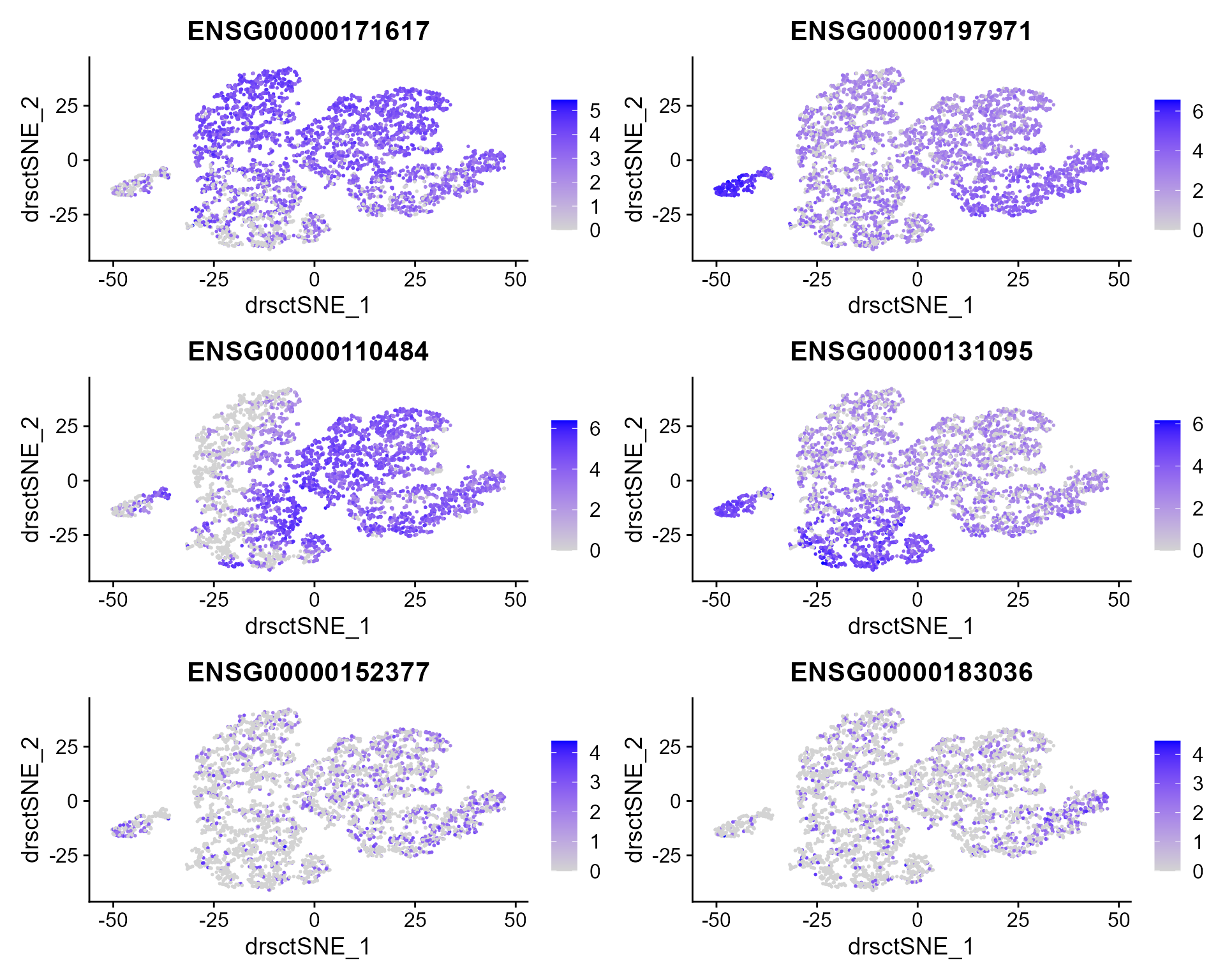
Dot plots
The size of the dot corresponds to the percentage of cells expressing the feature in each cluster. The color represents the average expression level
DotPlot(seus, features = genes)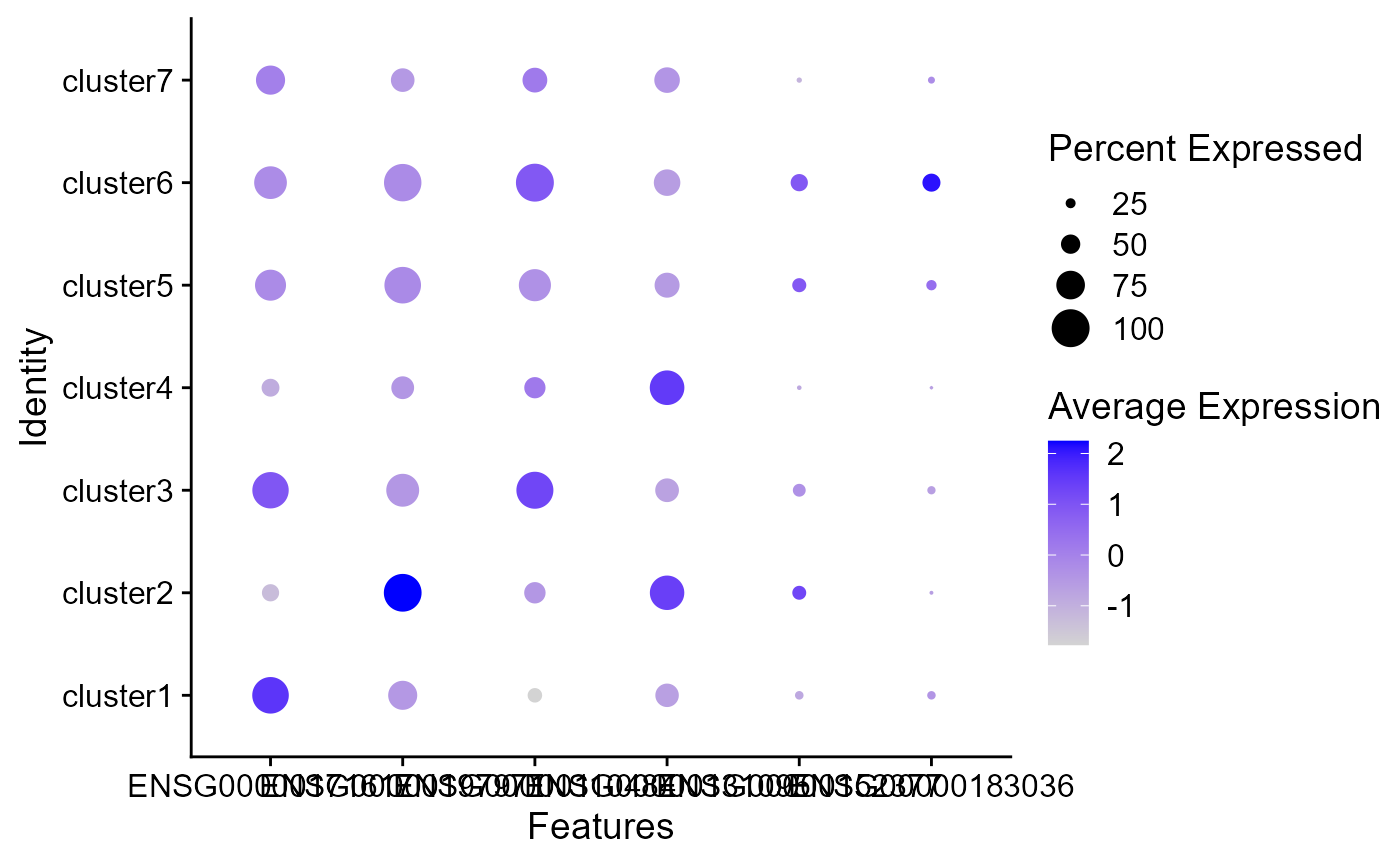
Heatmap plot
Single cell heatmap of feature expression
top20 <-  dat %>%
  group_by(cluster) %>%
  top_n(n = 20, wt = avg_log2FC)
genes <- top20$gene
# standard scaling (no regression)
seus <- ScaleData(seus)
#> Centering and scaling data matrix
DoHeatmap(subset(seus, downsample = 500), features = genes, size = 5)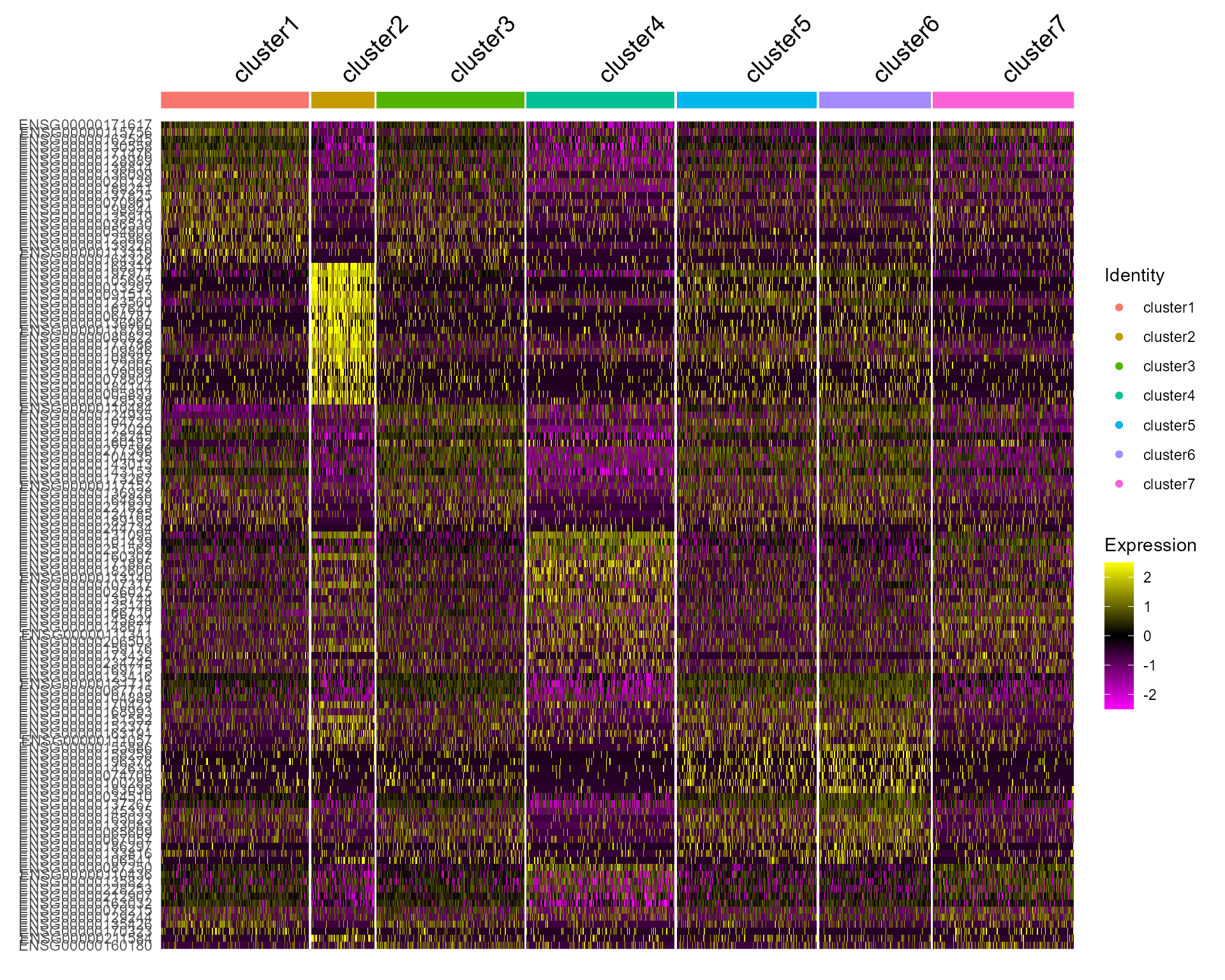
Fit DR-SC model using 480 spatially variable features and using MBIC to determine clusters
# choose spatially variable features
seus <- FindSVGs(seu, nfeatures = 480, verbose = F)
We set the argument variable.type=‘SVGs’ (default option) to use the spatially variable genes.
### Given K
seus <- DR.SC(seus, K=3:9, platform = 'Visium', verbose=F)
#> Neighbors were identified for 4634 out of 4634 spots.
#> Fit DR-SC model...
#> Using accurate PCA to obtain initial values
#> Starting parallel computing intial values...
#> Finish DR-SC model fitting
Plot the MBIC curve
seus <- selectModel(seus, pen.const = 0.8)
mbicPlot(seus)
Show the spatial scatter plot for clusters
spatialPlotClusters(seus)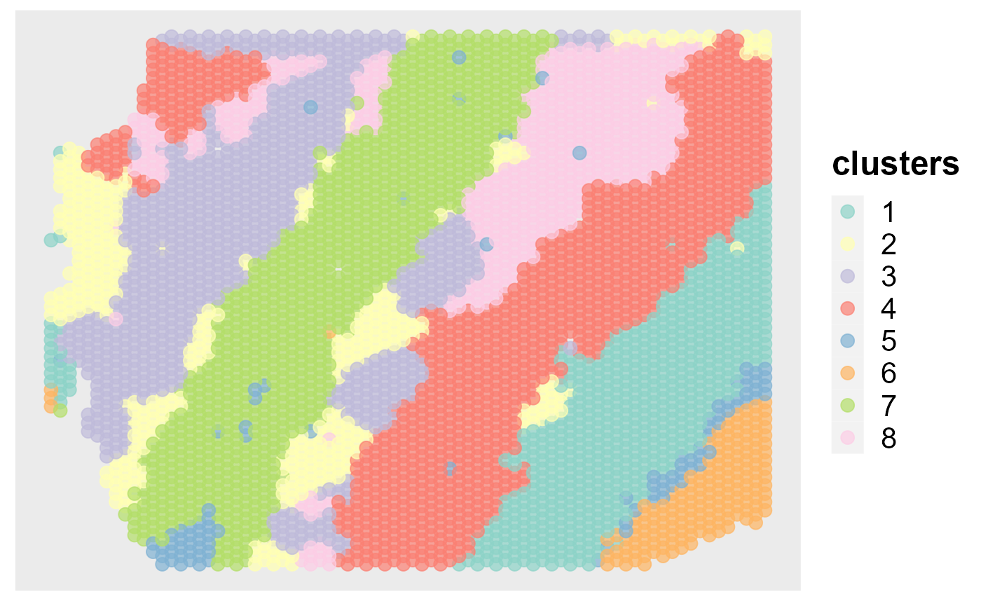
Show the tSNE plot based on the extracted features from DR-SC.
drscPlot(seus, dims=1:10)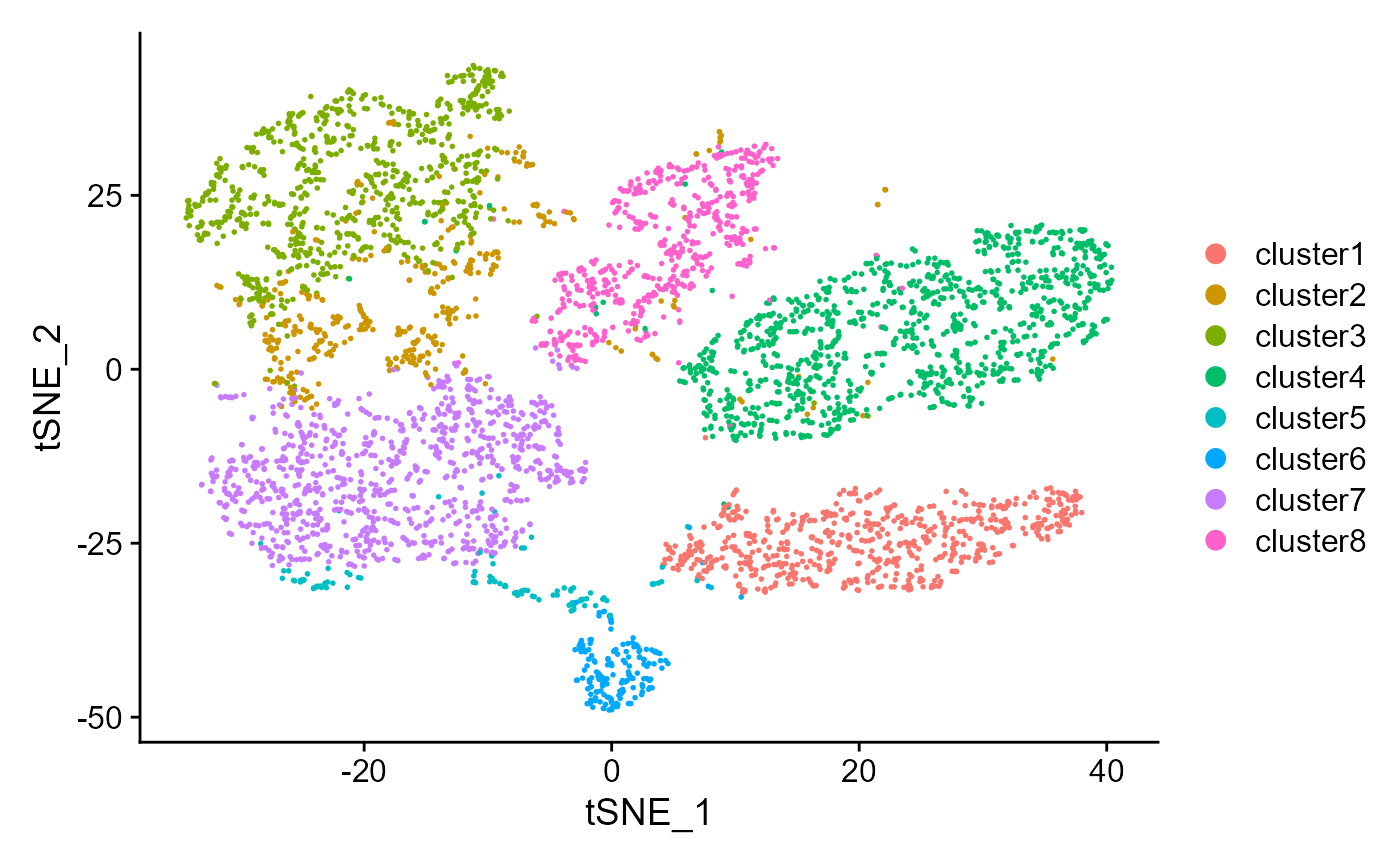
Session information
sessionInfo()
#> R version 4.4.1 (2024-06-14 ucrt)
#> Platform: x86_64-w64-mingw32/x64
#> Running under: Windows 11 x64 (build 26100)
#>
#> Matrix products: default
#>
#>
#> locale:
#> [1] LC_COLLATE=Chinese (Simplified)_China.utf8
#> [2] LC_CTYPE=Chinese (Simplified)_China.utf8
#> [3] LC_MONETARY=Chinese (Simplified)_China.utf8
#> [4] LC_NUMERIC=C
#> [5] LC_TIME=Chinese (Simplified)_China.utf8
#>
#> time zone: Asia/Shanghai
#> tzcode source: internal
#>
#> attached base packages:
#> [1] parallel  stats     graphics  grDevices utils     datasets  methods
#> [8] base
#>
#> other attached packages:
#> [1] dplyr_1.1.4           Seurat_5.1.0          SeuratObject_5.0.2
#> [4] sp_2.1-4              DR.SC_3.4             spatstat.geom_3.3-3
#> [7] spatstat.univar_3.0-1 spatstat.data_3.1-2
#>
#> loaded via a namespace (and not attached):
#>   [1] RColorBrewer_1.1-3     rstudioapi_0.16.0      jsonlite_1.8.9
#>   [4] magrittr_2.0.3         ggbeeswarm_0.7.2       spatstat.utils_3.1-0
#>   [7] farver_2.1.2           rmarkdown_2.28         fs_1.6.4
#>  [10] ragg_1.3.3             vctrs_0.6.5            ROCR_1.0-11
#>  [13] spatstat.explore_3.3-2 CompQuadForm_1.4.3     htmltools_0.5.8.1
#>  [16] sass_0.4.9             sctransform_0.4.1      parallelly_1.38.0
#>  [19] KernSmooth_2.23-24     bslib_0.8.0            htmlwidgets_1.6.4
#>  [22] desc_1.4.3             ica_1.0-3              plyr_1.8.9
#>  [25] plotly_4.10.4          zoo_1.8-12             cachem_1.1.0
#>  [28] igraph_2.0.3           mime_0.12              lifecycle_1.0.4
#>  [31] pkgconfig_2.0.3        Matrix_1.7-0           R6_2.5.1
#>  [34] fastmap_1.2.0          fitdistrplus_1.2-1     future_1.34.0
#>  [37] shiny_1.9.1            digest_0.6.37          colorspace_2.1-1
#>  [40] patchwork_1.3.0        S4Vectors_0.42.1       tensor_1.5
#>  [43] RSpectra_0.16-2        irlba_2.3.5.1          textshaping_0.4.0
#>  [46] labeling_0.4.3         progressr_0.14.0       fansi_1.0.6
#>  [49] spatstat.sparse_3.1-0  httr_1.4.7             polyclip_1.10-7
#>  [52] abind_1.4-8            compiler_4.4.1         withr_3.0.1
#>  [55] fastDummies_1.7.4      highr_0.11             MASS_7.3-60.2
#>  [58] tools_4.4.1            vipor_0.4.7            lmtest_0.9-40
#>  [61] beeswarm_0.4.0         httpuv_1.6.15          future.apply_1.11.2
#>  [64] goftest_1.2-3          glue_1.7.0             nlme_3.1-164
#>  [67] promises_1.3.0         grid_4.4.1             Rtsne_0.17
#>  [70] cluster_2.1.6          reshape2_1.4.4         generics_0.1.3
#>  [73] gtable_0.3.5           tidyr_1.3.1            data.table_1.16.0
#>  [76] utf8_1.2.4             BiocGenerics_0.50.0    RcppAnnoy_0.0.22
#>  [79] ggrepel_0.9.6          RANN_2.6.2             pillar_1.9.0
#>  [82] stringr_1.5.1          limma_3.58.1           spam_2.10-0
#>  [85] RcppHNSW_0.6.0         later_1.3.2            splines_4.4.1
#>  [88] lattice_0.22-6         survival_3.6-4         deldir_2.0-4
#>  [91] tidyselect_1.2.1       miniUI_0.1.1.1         pbapply_1.7-2
#>  [94] knitr_1.48             gridExtra_2.3          scattermore_1.2
#>  [97] stats4_4.4.1           xfun_0.47              statmod_1.5.0
#> [100] matrixStats_1.4.1      stringi_1.8.4          lazyeval_0.2.2
#> [103] yaml_2.3.10            evaluate_1.0.0         codetools_0.2-20
#> [106] tibble_3.2.1           cli_3.6.3              uwot_0.2.2
#> [109] xtable_1.8-4           reticulate_1.39.0      systemfonts_1.1.0
#> [112] munsell_0.5.1          jquerylib_0.1.4        Rcpp_1.0.13
#> [115] globals_0.16.3         spatstat.random_3.3-2  png_0.1-8
#> [118] ggrastr_1.0.2          pkgdown_2.1.1          ggplot2_3.5.2
#> [121] presto_1.0.0           dotCall64_1.1-1        mclust_6.1.1
#> [124] listenv_0.9.1          viridisLite_0.4.2      scales_1.3.0
#> [127] ggridges_0.5.6         leiden_0.4.3.1         purrr_1.0.2
#> [130] rlang_1.1.4            cowplot_1.1.3