GFM: A Simple Transcriptomics Data

Load real data

First, we load the ‘GFM’ package and the real data which can be downloaded here. This data is in the format of ‘.Rdata’ that inludes a gene expression matrix ‘X’ with 3460 rows (cells) and 2000 columns (genes), a vector ‘group’ specifying two groups of variable types (‘type’ variable) including ‘gaussian’ and ‘poisson’ and a vector ‘y’ meaning the clusters of cells annotated by experts. We compare the performance of ‘GFM’ and ‘LFM’ in downstream clustering analysis based on the benchchmarked clusters ‘y’.

githubURL <- "https://github.com/feiyoung/GFM/blob/main/vignettes_data/Brain76.Rdata?raw=true"
download.file(githubURL,"Brain76.Rdata",mode='wb')

Then load to R

load("Brain76.Rdata")
XList <- list(X[,group==1], X[,group==2])
types <- type
str(XList)
#> List of 2
#>  $ : num [1:3460, 1:1000] 0 0 0 0 0 ...
#>   ..- attr(*, "dimnames")=List of 2
#>   .. ..$ : chr [1:3460] "AAACAAGTATCTCCCA-1" "AAACAATCTACTAGCA-1" "AAACACCAATAACTGC-1" "AAACAGAGCGACTCCT-1" ...
#>   .. ..$ : chr [1:1000] "logcount_ENSG00000187608" "logcount_ENSG00000179403" "logcount_ENSG00000162408" "logcount_ENSG00000049245" ...
#>  $ : num [1:3460, 1:1000] 0 0 0 0 0 0 0 0 0 2 ...
#>   ..- attr(*, "dimnames")=List of 2
#>   .. ..$ : chr [1:3460] "AAACAAGTATCTCCCA-1" "AAACAATCTACTAGCA-1" "AAACACCAATAACTGC-1" "AAACAGAGCGACTCCT-1" ...
#>   .. ..$ : chr [1:1000] "count_ENSG00000187608" "count_ENSG00000179403" "count_ENSG00000162408" "count_ENSG00000049245" ...


library("GFM")
#> Loading required package: doSNOW
#> Loading required package: foreach
#> Loading required package: iterators
#> Loading required package: snow
#> Loading required package: parallel
#> 
#> Attaching package: 'parallel'
#> The following objects are masked from 'package:snow':
#> 
#>     clusterApply, clusterApplyLB, clusterCall, clusterEvalQ,
#>     clusterExport, clusterMap, clusterSplit, makeCluster, parApply,
#>     parCapply, parLapply, parRapply, parSapply, splitIndices,
#>     stopCluster
#> GFM :  Generalized factor model is implemented for ultra-high dimensional data with mixed-type variables.
#> Two algorithms, variational EM and alternate maximization, are designed to implement the generalized factor model,
#> respectively. The factor matrix and loading matrix together with the number of factors can be well estimated.
#> This model can be employed in social and behavioral sciences, economy and finance, and  genomics,
#> to extract interpretable nonlinear factors. More details can be referred to
#> Wei Liu, Huazhen Lin, Shurong Zheng and Jin Liu. (2021) <doi:10.1080/01621459.2021.1999818>.   Check out our Package website (https://feiyoung.github.io/GFM/docs/index.html) for a more complete description of the methods and analyses
#load("vignettes_data\\Brain76.Rdata")
#ls() # check the variables
set.seed(2023) # set a random seed for reproducibility.

Fit GFM model

We fit the GFM model using ‘gfm’ function.

q <- 15
system.time(
  gfm1 <- gfm(XList, types, q= q, verbose = TRUE)
)
#> Starting the varitional EM algorithm...
#> iter = 2, ELBO= -3750461.822684, dELBO=0.998254 
#> iter = 3, ELBO= -3554311.076859, dELBO=0.052300 
#> iter = 4, ELBO= -3415402.198187, dELBO=0.039082 
#> iter = 5, ELBO= -3306452.039078, dELBO=0.031900 
#> iter = 6, ELBO= -3217346.647111, dELBO=0.026949 
#> iter = 7, ELBO= -3142460.123095, dELBO=0.023276 
#> iter = 8, ELBO= -3078271.159787, dELBO=0.020426 
#> iter = 9, ELBO= -3022409.845541, dELBO=0.018147 
#> iter = 10, ELBO= -2973199.625335, dELBO=0.016282 
#> iter = 11, ELBO= -2929410.835170, dELBO=0.014728 
#> iter = 12, ELBO= -2890115.681500, dELBO=0.013414 
#> iter = 13, ELBO= -2854597.557781, dELBO=0.012290 
#> iter = 14, ELBO= -2822292.009491, dELBO=0.011317 
#> iter = 15, ELBO= -2792747.001267, dELBO=0.010468 
#> iter = 16, ELBO= -2765595.355226, dELBO=0.009722 
#> iter = 17, ELBO= -2740535.120688, dELBO=0.009061 
#> iter = 18, ELBO= -2717315.275484, dELBO=0.008473 
#> iter = 19, ELBO= -2695725.110295, dELBO=0.007945 
#> iter = 20, ELBO= -2675586.217373, dELBO=0.007471 
#> iter = 21, ELBO= -2656746.357345, dELBO=0.007041 
#> iter = 22, ELBO= -2639074.702982, dELBO=0.006652 
#> iter = 23, ELBO= -2622458.107292, dELBO=0.006296 
#> iter = 24, ELBO= -2606798.143554, dELBO=0.005971 
#> iter = 25, ELBO= -2592008.733701, dELBO=0.005673 
#> iter = 26, ELBO= -2578014.230523, dELBO=0.005399 
#> iter = 27, ELBO= -2564747.853111, dELBO=0.005146 
#> iter = 28, ELBO= -2552150.400275, dELBO=0.004912 
#> iter = 29, ELBO= -2540169.184545, dELBO=0.004695 
#> iter = 30, ELBO= -2528757.142764, dELBO=0.004493
#> Finish the varitional EM algorithm...
#>    user  system elapsed 
#>   93.61    5.28  152.44

Compare with LFM in downstream analysis

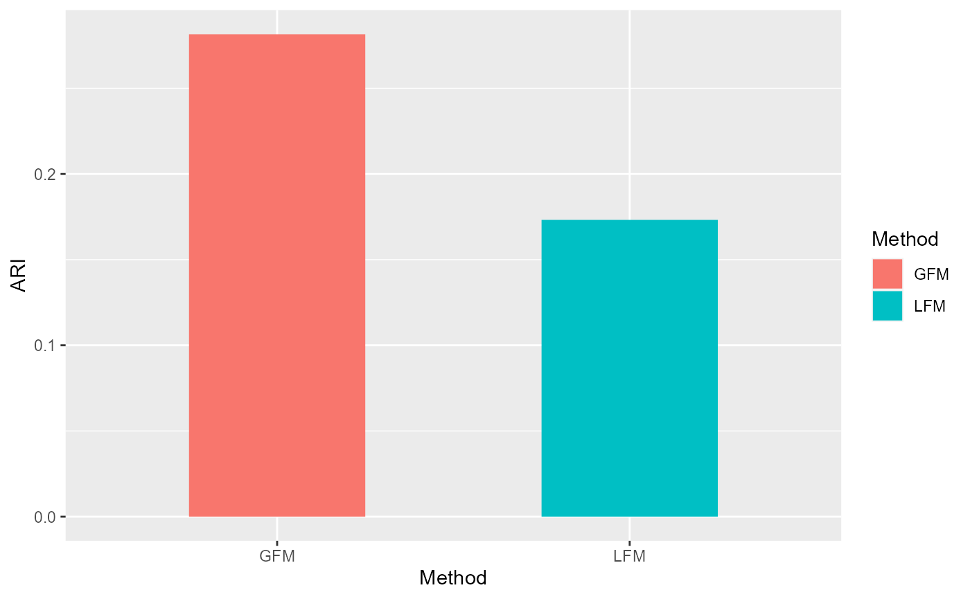
We conduct the clustering analysis based on the extracted factors by GFM and evaluate the adjusted rand index (ARI) value based on the annotated cluster labels by experts.

hH <- gfm1$hH
library(mclust)
#> Warning: package 'mclust' was built under R version 4.1.3
#> Package 'mclust' version 5.4.10
#> Type 'citation("mclust")' for citing this R package in publications.
set.seed(1)
gmm1 <- Mclust(hH, G=7)
ARI_gfm <- adjustedRandIndex(gmm1$classification, y)

We fit linear factor model using same number of factors.

fac <- Factorm(X, q=15)
hH_lfm <- fac$hH
set.seed(1)
gmm2 <- Mclust(hH_lfm, G=7)
ARI_lfm <- adjustedRandIndex(gmm2$classification, y)

Compare with the ARIs by visualization.

library(ggplot2)
#> Warning: package 'ggplot2' was built under R version 4.1.3
df1 <- data.frame(ARI= c(ARI_gfm,ARI_lfm),
                    Method =factor(c('GFM', "LFM")))
ggplot(data=df1, aes(x=Method, y=ARI, fill=Method)) + geom_bar(position = "dodge", stat="identity",width = 0.5)

Wei Liu

2023-06-24

Load real data

Fit GFM model

Compare with LFM in downstream analysis