OverGFM: simulated examples
Jinyu Nie, Zhilong Qin, Wei Liu
2023-08-10
Source:vignettes/OverGFM_exam.Rmd
OverGFM_exam.RmdIn this tutorial, we show the usage of the overdispersed generalized factor model (OverGFM) and compare it with the competitors.
Load GFM package
The package can be loaded with the following command:
## Loading required package: doSNOW## Loading required package: foreach## Loading required package: iterators## Loading required package: snow## Loading required package: parallel##
## Attaching package: 'parallel'## The following objects are masked from 'package:snow':
##
## clusterApply, clusterApplyLB, clusterCall, clusterEvalQ,
## clusterExport, clusterMap, clusterSplit, makeCluster, parApply,
## parCapply, parLapply, parRapply, parSapply, splitIndices,
## stopCluster## GFM : Generalized factor model is implemented for ultra-high dimensional data with mixed-type variables.
## Two algorithms, variational EM and alternate maximization, are designed to implement the generalized factor model,
## respectively. The factor matrix and loading matrix together with the number of factors can be well estimated.
## This model can be employed in social and behavioral sciences, economy and finance, and genomics,
## to extract interpretable nonlinear factors. More details can be referred to
## Wei Liu, Huazhen Lin, Shurong Zheng and Jin Liu. (2021) <doi:10.1080/01621459.2021.1999818>. Check out our Package website (https://feiyoung.github.io/GFM/docs/index.html) for a more complete description of the methods and analysesLoad rrpack and PCAmixdata packages for other methods
The rrpack package can be loaded with the following command:
library("rrpack")The PCAmixdata package can be loaded with the following command:
library("PCAmixdata")## Warning: package 'PCAmixdata' was built under R version 4.1.3Introduction to the data generation mechanisms
We define the function with details for the data generation mechanism.
gendata_s2 <- function (seed = 1, n = 500, p = 500,
                        type =  c('homonorm', 'heternorm', 'pois', 'bino', 'norm_pois',
                                  'pois_bino', 'npb'),
                        q = 6, rho = c(0.05, 0.2, 0.1), n_bin=1, sigma_eps=0.1){
  library(MASS)
  Diag <- GFM:::Diag
  cor.mat <- GFM:::cor.mat
  type <- match.arg(type)
  rho_gauss <- rho[1]
  rho_pois <- rho[2]
  rho_binary <- rho[3]
  set.seed(seed)
  Z <- matrix(rnorm(p * q), p, q)
  if (type == "homonorm") {
    g1 <- 1:p
    Z <- rho_gauss * Z
  }else if (type == "heternorm"){
    g1 <- 1:p
    Z <- rho_gauss * Z
  }else if(type == "pois"){
    g1 <- 1:p
    Z <- rho_pois * Z
  }else if(type == 'bino'){
    g1 <- 1:p
    Z <- rho_binary * Z
  }else if (type == "norm_pois") {
    g1 <- 1:floor(p/2)
    g2 <- (floor(p/2) + 1):p
    Z[g1, ] <- rho_gauss * Z[g1, ]
    Z[g2, ] <- rho_pois * Z[g2, ]
  }else if (type == "pois_bino") {
    g1 <- 1:floor(p/2)
    g2 <- (floor(p/2) + 1):p

    Z[g1, ] <- rho_pois * Z[g1, ]
    Z[g2, ] <- rho_binary * Z[g2, ]
  }else if(type == 'npb'){
    g1 <- 1:floor(p/3)
    g2 <- (floor(p/3) + 1):floor(p*2/3)
    g3 <- (floor(2*p/3) + 1):p
    Z[g1, ] <- rho_gauss * Z[g1, ]
    Z[g2, ] <- rho_pois * Z[g2, ]
    Z[g3, ] <- rho_binary * Z[g3, ]
  }
  svdZ <- svd(Z)
  B1 <- svdZ$u %*% Diag(svdZ$d[1:q])
  B0 <- B1 %*% Diag(sign(B1[1, ]))
  mu0 <- 0.4 * rnorm(p)
  Bm0 <- cbind(mu0, B0)

  set.seed(seed)
  H <- mvrnorm(n, mu = rep(0, q), cor.mat(q, 0.5))
  svdH <- svd(cov(H))
  H0 <- scale(H, scale = F) %*% svdH$u %*% Diag(1/sqrt(svdH$d)) %*%
    svdH$v
  if (type == "homonorm") {
    X <- H0 %*% t(B0) + matrix(mu0, n, p, byrow = T) + mvrnorm(n,
                                                               rep(0, p), sigma_eps*diag(p))
    group <- rep(1, p)
    XList <- list(X)
    types <- c("gaussian")

  }else if (type == "heternorm") {
    sigmas = sigma_eps*(0.1 + 4 * runif(p))
    X <- H0 %*% t(B0) + matrix(mu0, n, p, byrow = T) + mvrnorm(n,
                                                               rep(0, p), diag(sigmas))
    group <- rep(1, p)

    XList <- list(X)
    types <- c("gaussian")

  }else if (type == "pois") {


    Eta <- H0 %*% t(B0) + matrix(mu0, n, p, byrow = T) + mvrnorm(n,rep(0, p),
                                                                 sigma_eps*diag(p))
    mu <- exp(Eta)
    X <- matrix(rpois(n * p, lambda = mu), n, p)
    group <- rep(1, p)
    XList <- list(X[,g1])
    types <- c("poisson")
  }else if(type == 'bino'){

    Eta <- cbind(1, H0) %*% t(Bm0[g1, ]) + mvrnorm(n,rep(0, p), sigma_eps*diag(p))
    mu <- 1/(1 + exp(-Eta))
    X <- matrix(rbinom(prod(dim(mu)), n_bin, mu), n, p)
    group <- rep(1, p)

    XList <- list(X[,g1])
    types <- c("binomial")
  }else if (type == "norm_pois") {

    Eps <- mvrnorm(n,rep(0, p), sigma_eps*diag(p))
    mu1 <- cbind(1, H0) %*% t(Bm0[g1, ]) + Eps[, g1]
    mu2 <- exp(cbind(1, H0) %*% t(Bm0[g2, ])+ Eps[, g2])
    X <- cbind(matrix(rnorm(prod(dim(mu1)), mu1, 1), n, floor(p/2)),
               matrix(rpois(prod(dim(mu2)), mu2), n, ncol(mu2)))
    group <- c(rep(1, length(g1)), rep(2, length(g2)))

    XList <- list(X[,g1], X[,g2])
    types <- c("gaussian", "poisson")

  }else if (type == "pois_bino") {

    Eps <- mvrnorm(n,rep(0, p), sigma_eps*diag(p))
    mu1 <- exp(cbind(1, H0) %*% t(Bm0[g1, ])+ Eps[,g1])
    mu2 <- 1/(1 + exp(-cbind(1, H0) %*% t(Bm0[g2, ])- Eps[,g2]))
    X <- cbind(matrix(rpois(prod(dim(mu1)), mu1), n, ncol(mu1)),
               matrix(rbinom(prod(dim(mu2)), n_bin, mu2), n, ncol(mu2)))
    group <- c(rep(1, length(g1)), rep(2, length(g2)))
    XList <- list(X[,g1], X[,g2])
    types <- c("poisson", 'binomial')
  }else if(type == 'npb'){

    Eps <- mvrnorm(n,rep(0, p), sigma_eps*diag(p))
    mu11 <- cbind(1, H0) %*% t(Bm0[g1, ]) + Eps[,g1]
    mu1 <- exp(cbind(1, H0) %*% t(Bm0[g2, ]) +  Eps[,g2])
    mu2 <- 1/(1 + exp(-cbind(1, H0) %*% t(Bm0[g3, ])-  Eps[,g3]))
    X <- cbind(matrix(rnorm(prod(dim(mu11)),mu11, 1), n, ncol(mu11)),
               matrix(rpois(prod(dim(mu1)), mu1), n, ncol(mu1)),
               matrix(rbinom(prod(dim(mu2)), n_bin, mu2), n, ncol(mu2)))
    group <- c(rep(1, length(g1)), rep(2, length(g2)), rep(3, length(g3)))
    XList <- list(X[,g1], X[,g2], X[,g3])
    types <- c("gaussian", "poisson", 'binomial')
  }

  return(list(X=X, XList = XList,  types= types, B0 = B0, H0 = H0, mu0 = mu0))
}
Brief description of other methods
GFM method capable of handling mixed-type data is implemented in the R package \(\bf GFM\).
MRRR method which is implemented in the R package \(\bf rrpack\) also handles mixed-type data through reduced-rank regression model, and we redefine the function of this method and modify its output results for comparison conveniently.
Diag <- GFM:::Diag
## Compare with MRRR
mrrr_run <- function(Y, rank0,family=list(poisson()),
                     familygroup,  epsilon = 1e-4, sv.tol = 1e-2,lambdaSVD=0.1, maxIter = 2000, trace=TRUE){
  # epsilon = 1e-4; sv.tol = 1e-2; maxIter = 30; trace=TRUE

  require(rrpack)

  n <- nrow(Y); p <- ncol(Y)
  X <- cbind(1, diag(n))


  svdX0d1 <- svd(X)$d[1]
  init1 = list(kappaC0 = svdX0d1 * 5)
  offset = NULL
  control = list(epsilon = epsilon, sv.tol = sv.tol, maxit = maxIter,
                 trace = trace, gammaC0 = 1.1, plot.cv = TRUE,
                 conv.obj = TRUE)
  res_mrrr <- mrrr(Y=Y, X=X[,-1], family = family, familygroup = familygroup,
                   penstr = list(penaltySVD = "rankCon", lambdaSVD = lambdaSVD),
                   control = control, init = init1, maxrank = rank0)

  hmu <- res_mrrr$coef[1,]
  hTheta <- res_mrrr$coef[-1,]
  #print(dim(hTheta))
  # Matrix::rankMatrix(hTheta)
  svd_Theta <- svd(hTheta, nu=rank0,nv =rank0)
  hH <- svd_Theta$u
  hB <- svd_Theta$v %*% Diag(svd_Theta$d[1:rank0])
  #print(dim(svd_Theta$v))
  #print(dim(Diag(svd_Theta$d)))
  return(list(hH=hH, hB=hB, hmu= hmu))
}
PCAmix method which uses Principal component analysis for data with mix of qualitative and quantitative variables is implemented in the R package \(\bf PCAmixdata\).
LFM method which handles linear factor model is implemented in the R package \(\bf GFM\), and we define the function of this method based on R package \(\bf GFM\).
factorm <- function(X, q=NULL){

  signrevise <- GFM:::signrevise
  if ((!is.null(q)) && (q < 1))
    stop("q must be NULL or other positive integer!")
  if (!is.matrix(X))
    stop("X must be a matrix.")
  mu <- colMeans(X)
  X <- scale(X, scale = FALSE)
  n <- nrow(X)
  p <- ncol(X)
  if (p > n) {
    svdX <- eigen(X %*% t(X))
    evalues <- svdX$values
    eigrt <- evalues[1:(21 - 1)]/evalues[2:21]
    if (is.null(q)) {
      q <- which.max(eigrt)
    }
    hatF <- as.matrix(svdX$vector[, 1:q] * sqrt(n))
    B2 <- n^(-1) * t(X) %*% hatF
    sB <- sign(B2[1, ])
    hB <- B2 * matrix(sB, nrow = p, ncol = q, byrow = TRUE)
    hH <- sapply(1:q, function(k) hatF[, k] * sign(B2[1,
    ])[k])
  }
  else {
    svdX <- eigen(t(X) %*% X)
    evalues <- svdX$values
    eigrt <- evalues[1:(21 - 1)]/evalues[2:21]
    if (is.null(q)) {
      q <- which.max(eigrt)
    }
    hB1 <- as.matrix(svdX$vector[, 1:q])
    hH1 <- n^(-1) * X %*% hB1
    svdH <- svd(hH1)
    hH2 <- signrevise(svdH$u * sqrt(n), hH1)
    if (q == 1) {
      hB1 <- hB1 %*% svdH$d[1:q] * sqrt(n)
    }
    else {
      hB1 <- hB1 %*% diag(svdH$d[1:q]) * sqrt(n)
    }
    sB <- sign(hB1[1, ])
    hB <- hB1 * matrix(sB, nrow = p, ncol = q, byrow = TRUE)
    hH <- sapply(1:q, function(j) hH2[, j] * sB[j])
  }
  sigma2vec <- colMeans((X - hH %*% t(hB))^2)
  res <- list()
  res$hH <- hH
  res$hB <- hB
  res$mu <- mu
  res$q <- q
  res$sigma2vec <- sigma2vec
  res$propvar <- sum(evalues[1:q])/sum(evalues)
  res$egvalues <- evalues
  attr(res, "class") <- "fac"
  return(res)
}
OverGFM can handle overdispersed mixed-type data
First, we generate a simulated data for three mixed-type variables based on the aforementioned data generate function. We fix \((n,p) = (500,500)\) ,\(\sigma^2 = 0.7\) and the signal strength \((\rho_1, \rho_2, \rho_3)=(0.05,0.2,0.1)\). Additionally, we set the number of factor \(q\) is 6. The details for the data setting is following :
  q <- 6
  datList <- gendata_s2(seed = 1, type= 'npb', n=500, p=500, q=q,
                        rho= c(0.05, 0.2, 0.1) ,sigma_eps = 0.7)
Second, we define the trace statistic to assess the performance.
trace_statistic_fun <- function(H, H0){

  tr_fun <- function(x) sum(diag(x))
  mat1 <- t(H0) %*% H %*% ginv(t(H) %*% H) %*% t(H) %*% H0

  tr_fun(mat1) / tr_fun(t(H0) %*% H0)

}
Then we use OverGFM to fit model.
gfm_over <- overdispersedGFM(datList$XList, types=datList$types, q=q)## Starting the varitional EM algorithm for overdispersed GFM model...## iter = 2, ELBO= -252789.984137, dELBO=1.000000
## iter = 3, ELBO= -248772.765747, dELBO=0.015892
## iter = 4, ELBO= -247448.671589, dELBO=0.005323
## iter = 5, ELBO= -247118.751955, dELBO=0.001333
## iter = 6, ELBO= -247259.575933, dELBO=0.000570
## iter = 7, ELBO= -247619.692539, dELBO=0.001456
## iter = 8, ELBO= -248064.027932, dELBO=0.001794
## iter = 9, ELBO= -248522.208121, dELBO=0.001847
## iter = 10, ELBO= -248959.018478, dELBO=0.001758
## iter = 11, ELBO= -249358.036208, dELBO=0.001603
## iter = 12, ELBO= -249712.928954, dELBO=0.001423
## iter = 13, ELBO= -250022.764386, dELBO=0.001241
## iter = 14, ELBO= -250289.428472, dELBO=0.001067
## iter = 15, ELBO= -250516.182259, dELBO=0.000906
## iter = 16, ELBO= -250706.850224, dELBO=0.000761
## iter = 17, ELBO= -250865.366958, dELBO=0.000632
## iter = 18, ELBO= -250995.530564, dELBO=0.000519
## iter = 19, ELBO= -251100.876461, dELBO=0.000420
## iter = 20, ELBO= -251184.621466, dELBO=0.000334
## iter = 21, ELBO= -251249.648507, dELBO=0.000259
## iter = 22, ELBO= -251298.514286, dELBO=0.000194
## iter = 23, ELBO= -251333.469229, dELBO=0.000139
## iter = 24, ELBO= -251356.483332, dELBO=0.000092
## iter = 25, ELBO= -251369.274090, dELBO=0.000051
## iter = 26, ELBO= -251373.334277, dELBO=0.000016
## iter = 27, ELBO= -251369.958337, dELBO=0.000013
## iter = 28, ELBO= -251360.266742, dELBO=0.000039
## iter = 29, ELBO= -251345.228043, dELBO=0.000060
## iter = 30, ELBO= -251325.678570, dELBO=0.000078## Finish the varitional EM algorithm...Other methods poorly handle overdispersed mixed-type data
We use other methods to fit model.
  lfm <- factorm(datList$X, q=q)
  gfm_am <- gfm(datList$XList, types=datList$types, q=q, algorithm = "AM",
                maxIter = 15)
## Starting the two-step method with alternate maximization in the first step...## ---------- B updation is finished!---------## ---------- H updation is finished!---------## Iter=1, dB=1, dH=1.0279,dc=1, c=1.2604## ---------- B updation is finished!---------## ---------- H updation is finished!---------## Iter=2, dB=0.3023, dH=0.3047,dc=0.0039, c=1.2555## ---------- B updation is finished!---------## ---------- H updation is finished!---------## Iter=3, dB=0.5384, dH=0.8304,dc=0.0031, c=1.2593## ---------- B updation is finished!---------## ---------- H updation is finished!---------## Iter=4, dB=0.0981, dH=0.141,dc=0.0021, c=1.262## ---------- B updation is finished!---------## ---------- H updation is finished!---------## Iter=5, dB=0.0751, dH=0.1143,dc=0.0016, c=1.264## ---------- B updation is finished!---------## ---------- H updation is finished!---------## Iter=6, dB=0.0624, dH=0.0976,dc=0.0012, c=1.2655## ---------- B updation is finished!---------## ---------- H updation is finished!---------## Iter=7, dB=0.0542, dH=0.086,dc=0.001, c=1.2668## ---------- B updation is finished!---------## ---------- H updation is finished!---------## Iter=8, dB=0.0483, dH=0.0772,dc=8e-04, c=1.2678## ---------- B updation is finished!---------## ---------- H updation is finished!---------## Iter=9, dB=0.0439, dH=0.0705,dc=6e-04, c=1.2686## ---------- B updation is finished!---------## ---------- H updation is finished!---------## Iter=10, dB=0.0404, dH=0.0655,dc=5e-04, c=1.2692## ---------- B updation is finished!---------## ---------- H updation is finished!---------## Iter=11, dB=0.0378, dH=0.0617,dc=4e-04, c=1.2698## ---------- B updation is finished!---------## ---------- H updation is finished!---------## Iter=12, dB=0.0358, dH=0.0587,dc=4e-04, c=1.2703## ---------- B updation is finished!---------## ---------- H updation is finished!---------## Iter=13, dB=0.0342, dH=0.0563,dc=3e-04, c=1.2707## ---------- B updation is finished!---------## ---------- H updation is finished!---------## Iter=14, dB=0.0328, dH=0.054,dc=3e-04, c=1.2711## ---------- B updation is finished!---------## ---------- H updation is finished!---------## Iter=15, dB=0.0315, dH=0.0519,dc=3e-04, c=1.2714## Finish the two-step method
  familygroup <- lapply(1:length(datList$types), function(j) rep(j,                                                         ncol(datList$XList[[j]])))
  res_mrrr <- mrrr_run(datList$X, rank0=q, family=list(gaussian(), poisson(),
                                                       binomial()),familygroup =
                         unlist(familygroup), maxIter=2000)
## Doing generalized PCA...
## iter = 1 obj/Cnorm_diff = 443660.9
## iter = 2 obj/Cnorm_diff = 427453.7
## iter = 3 obj/Cnorm_diff = 422871.2
## iter = 4 obj/Cnorm_diff = 417838.6
## iter = 5 obj/Cnorm_diff = 412486.6
## iter = 6 obj/Cnorm_diff = 407046
## iter = 7 obj/Cnorm_diff = 401854.1
## iter = 8 obj/Cnorm_diff = 397307.5
## iter = 9 obj/Cnorm_diff = 393733.3
## iter = 10 obj/Cnorm_diff = 391228.2
## iter = 11 obj/Cnorm_diff = 389618.6
## iter = 12 obj/Cnorm_diff = 388597.5
## iter = 13 obj/Cnorm_diff = 387890.7
## iter = 14 obj/Cnorm_diff = 387334.3
## iter = 15 obj/Cnorm_diff = 386860.5
## iter = 16 obj/Cnorm_diff = 386447.7
## iter = 17 obj/Cnorm_diff = 386082.9
## iter = 18 obj/Cnorm_diff = 385747.8
## iter = 19 obj/Cnorm_diff = 385419.1
## iter = 20 obj/Cnorm_diff = 385073.6
## iter = 21 obj/Cnorm_diff = 384693.8
## iter = 22 obj/Cnorm_diff = 384348.9
## iter = 22 obj/Cnorm_diff = 384348.9
## iter = 23 obj/Cnorm_diff = 384300.1
## iter = 24 obj/Cnorm_diff = 384261.5
  dat_bino <- as.data.frame(datList$XList[[3]])
  for(jj in 1:ncol(dat_bino)) dat_bino[,jj] <- factor(dat_bino[,jj])
  dat_norm <- as.data.frame(cbind(datList$XList[[1]],datList$XList[[2]]))
  res_pcamix <- PCAmix(X.quanti = dat_norm, X.quali = dat_bino,rename.level=TRUE, ndim=q,
                       graph=F)
  reslits <- lapply(res_pcamix$coef, function(x) x[c(seq(2, ncol(dat_norm)+1, by=1),
                                                     seq(ncol(dat_norm)+3,
                                                         nrow(res_pcamix$coef[[1]]), by=2)),])
  loadings <- Reduce(cbind, reslits)
  GFM_H <- trace_statistic_fun(gfm_am$hH, datList$H0)
  GFM_G <- trace_statistic_fun(cbind(gfm_am$hmu,gfm_am$hB),
                                    cbind(datList$mu0,datList$B0))
  MRRR_H <- trace_statistic_fun(res_mrrr$hH, datList$H0)
  MRRR_G <- trace_statistic_fun(cbind(res_mrrr$hmu,res_mrrr$hB),
                                     cbind(datList$mu0,datList$B0))
  PCAmix_H <- trace_statistic_fun(res_pcamix$ind$coord, datList$H0)
  PCAmix_G <- trace_statistic_fun(loadings, cbind(datList$mu0,datList$B0))
  LFM_H <- trace_statistic_fun(lfm$hH, datList$H0)
  LFM_G <- trace_statistic_fun(cbind(lfm$mu,lfm$hB), cbind(datList$mu0,datList$B0))
Visualization
We visualize the comparison of the trace statistic of \(\bf H\) and \(\bf \Upsilon\) for each methods
## Warning: package 'ggplot2' was built under R version 4.1.3
value <- c(OverGFM_H,OverGFM_G,GFM_H,GFM_G,MRRR_H,MRRR_G,PCAmix_H,PCAmix_G,LFM_H,LFM_G)
df <- data.frame(Value = value,
                 Methods = factor(rep(c("OverGFM","GFM","MRRR","PCAmix","LFM"), each = 2),
                                  levels = c("OverGFM","GFM","MRRR","PCAmix","LFM")),
                 Trace = factor(rep(c("Tr_H","Tr_Gamma"), times = 5),levels = c("Tr_H","Tr_Gamma")))
ggplot(data = df,aes(x = Methods, y = Value, colour = Methods, fill=Methods)) +
  geom_bar(stat="identity") +
  facet_grid(Trace ~ .,drop = TRUE, scales = "free_x") + theme_bw() +
  theme(axis.text.x = element_text(size = 10,angle = 25, hjust = 1, vjust = 1),
        axis.text.y = element_text(size = 10, hjust = 1, vjust = 1),
        axis.title.x = element_text(size = 15),
        axis.title.y = element_text(size = 15),
        legend.title=element_blank())+
  labs( x="Method", y = "Trace statistic ")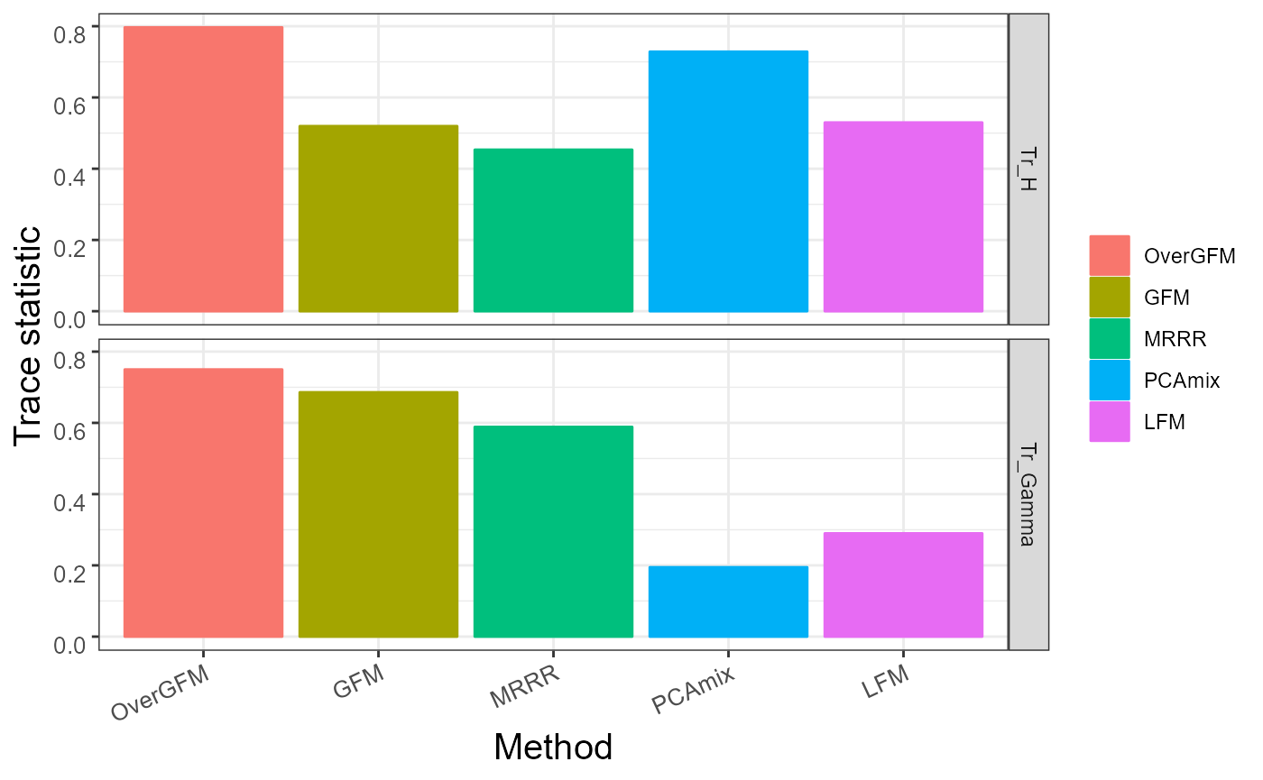
Session information
## R version 4.1.2 (2021-11-01)
## Platform: x86_64-w64-mingw32/x64 (64-bit)
## Running under: Windows 10 x64 (build 22621)
##
## Matrix products: default
##
## locale:
## [1] LC_COLLATE=Chinese (Simplified)_China.936
## [2] LC_CTYPE=Chinese (Simplified)_China.936
## [3] LC_MONETARY=Chinese (Simplified)_China.936
## [4] LC_NUMERIC=C
## [5] LC_TIME=Chinese (Simplified)_China.936
##
## attached base packages:
## [1] parallel  stats     graphics  grDevices utils     datasets  methods
## [8] base
##
## other attached packages:
## [1] ggplot2_3.4.1    MASS_7.3-55      PCAmixdata_3.1   rrpack_0.1-11
## [5] GFM_1.2.1        doSNOW_1.0.20    snow_0.4-4       iterators_1.0.14
## [9] foreach_1.5.2
##
## loaded via a namespace (and not attached):
##  [1] Rcpp_1.0.10           lattice_0.20-45       assertthat_0.2.1
##  [4] glmnet_4.1-3          rprojroot_2.0.3       digest_0.6.29
##  [7] utf8_1.2.3            R6_2.5.1              evaluate_0.15
## [10] highr_0.9             pillar_1.9.0          rlang_1.1.0
## [13] rstudioapi_0.13       irlba_2.3.5           jquerylib_0.1.4
## [16] Matrix_1.4-0          rmarkdown_2.11        pkgdown_2.0.6
## [19] labeling_0.4.2        textshaping_0.3.6     desc_1.4.0
## [22] splines_4.1.2         stringr_1.4.0         munsell_0.5.0
## [25] compiler_4.1.2        xfun_0.29             pkgconfig_2.0.3
## [28] systemfonts_1.0.4     shape_1.4.6           htmltools_0.5.2
## [31] tidyselect_1.1.2      tibble_3.2.1          lassoshooting_0.1.5-1
## [34] codetools_0.2-18      fansi_1.0.4           withr_2.5.0
## [37] crayon_1.5.1          dplyr_1.0.9           grid_4.1.2
## [40] jsonlite_1.8.0        gtable_0.3.3          lifecycle_1.0.3
## [43] DBI_1.1.2             magrittr_2.0.3        scales_1.2.1
## [46] cli_3.2.0             stringi_1.7.6         cachem_1.0.6
## [49] farver_2.1.1          fs_1.5.2              bslib_0.3.1
## [52] ragg_1.2.2            vctrs_0.6.1           generics_0.1.2
## [55] tools_4.1.2           glue_1.6.2            purrr_0.3.4
## [58] fastmap_1.1.0         survival_3.2-13       yaml_2.3.6
## [61] colorspace_2.1-0      memoise_2.0.1         knitr_1.37
## [64] sass_0.4.1