This vignette introduces the FAST workflow for the analysis of two humn dorsolateral prefrontal cortex (DLPFC) spatial transcriptomics dataset. FAST workflow is based on the PRECASTObj object created in the PRECAST R package and the workflow of FAST is similar to that of PRECAST; see the vignette (https://feiyoung.github.io/PRECAST/articles/PRECAST.BreastCancer.html) for the workflow of PRECAST. In this vignette, the workflow of FAST consists of three steps
- Independent preprocessing and model setting
- Spatial dimension reduction using FAST
- Downstream analysis (i.e. , embedding alignment and spatial clustering using iSC-MEB, visualization of clusters and embeddings, remove unwanted variation, combined differential expression analysis)
- Except for the above downstream analyses, cell-cell interaction analysis and trajectory inference can also be performed on the basis of the embeddings obtained by FAST.
We demonstrate the use of FAST to two DLPFC Visium data that are here, which can be downloaded to the current working path by the following command:
githubURL <- "https://github.com/feiyoung/FAST/blob/main/vignettes_data/seulist2_ID9_10.RDS?raw=true"
download.file(githubURL,"seulist2_ID9_10.RDS",mode='wb')
Then load to R
dlpfc2 <- readRDS("./seulist2_ID9_10.RDS")The package can be loaded with the command:
library(ProFAST) # load the package of FAST method
#> Loading required package: gtools
#>
#>
library(PRECAST)
#> Loading required package: parallel
#> PRECAST :  An efficient data integration method is provided for multiple spatial transcriptomics data with non-cluster-relevant effects such as the complex batch effects. It unifies spatial factor analysis simultaneously with spatial clustering and embedding alignment, requiring only partially shared cell/domain clusters across datasets. More details can be referred to Wei Liu, et al. (2023) <doi:10.1038/s41467-023-35947-w>.   Check out our Package website (https://feiyoung.github.io/PRECAST/index.html) for a more complete description of the methods and analyses
library(Seurat)
#> Warning: package 'Seurat' was built under R version 4.1.3
#> Attaching SeuratObject
#> Attaching sp
View the DLPFC data
First, we view the the two spatial transcriptomics data with ST platform. There are ~15000 genes for each data batch and ~7000 spots in total.
dlpfc2 ## a list including three Seurat object with default assay: RNA
#> [[1]]
#> An object of class Seurat
#> 15027 features across 3639 samples within 1 assay
#> Active assay: RNA (15027 features, 2000 variable features)
#>
#> [[2]]
#> An object of class Seurat
#> 15809 features across 3673 samples within 1 assay
#> Active assay: RNA (15809 features, 2000 variable features)
Check the content in dlpfc2.
head(dlpfc2[[1]])We observed the genes are Ensembl IDs. In the following, we will transfer the Ensembl IDs to gene symbols for matching the housekeeping genes in the downstream analysis for removing the unwanted variations.
row.names(dlpfc2[[1]])[1:10]Create a PRECASTObject object
We show how to create a PRECASTObject object step by step. First, we create a Seurat list object using the count matrix and meta data of each data batch.
- Note: the spatial coordinates must be contained in the meta data and named as
rowandcol, which benefits the identification of spaital coordinates by FAST
## Get the gene-by-spot read count matrices
countList <- lapply(dlpfc2, function(x) x[["RNA"]]@counts)
M <- length(countList)
### transfer the Ensembl ID to symbol
for(r in 1:M){
row.names(countList[[r]]) <- transferGeneNames(row.names(countList[[r]]), now_name = "ensembl",
to_name="symbol",
species="Human", Method='eg.db')
}
#> 'select()' returned 1:many mapping between keys and columns
#> 'select()' returned 1:many mapping between keys and columns
## Check the spatial coordinates: Yes, they are named as "row" and "col"!
print(head(dlpfc2[[1]]@meta.data))
#> orig.ident nCount_RNA nFeature_RNA barcode
#> AAACAAGTATCTCCCA-1 SeuratProject 8436 3564 AAACAAGTATCTCCCA-1
#> AAACAATCTACTAGCA-1 SeuratProject 1662 1145 AAACAATCTACTAGCA-1
#> AAACACCAATAACTGC-1 SeuratProject 3758 1949 AAACACCAATAACTGC-1
#> AAACAGAGCGACTCCT-1 SeuratProject 5418 2409 AAACAGAGCGACTCCT-1
#> AAACAGCTTTCAGAAG-1 SeuratProject 4262 2248 AAACAGCTTTCAGAAG-1
#> AAACAGGGTCTATATT-1 SeuratProject 3984 2159 AAACAGGGTCTATATT-1
#> sample_name tissue row col imagerow imagecol Cluster height
#> AAACAAGTATCTCCCA-1 151673 1 50 102 381.0981 440.6391 7 600
#> AAACAATCTACTAGCA-1 151673 1 3 43 126.3276 259.6310 4 600
#> AAACACCAATAACTGC-1 151673 1 59 19 427.7678 183.0783 8 600
#> AAACAGAGCGACTCCT-1 151673 1 14 94 186.8137 417.2367 6 600
#> AAACAGCTTTCAGAAG-1 151673 1 43 9 341.2691 152.7003 3 600
#> AAACAGGGTCTATATT-1 151673 1 47 13 362.9163 164.9415 3 600
#> width sum_umi sum_gene subject position replicate
#> AAACAAGTATCTCCCA-1 600 8458 3586 Br8100 0 1
#> AAACAATCTACTAGCA-1 600 1667 1150 Br8100 0 1
#> AAACACCAATAACTGC-1 600 3769 1960 Br8100 0 1
#> AAACAGAGCGACTCCT-1 600 5433 2424 Br8100 0 1
#> AAACAGCTTTCAGAAG-1 600 4278 2264 Br8100 0 1
#> AAACAGGGTCTATATT-1 600 4004 2178 Br8100 0 1
#> subject_position discard key
#> AAACAAGTATCTCCCA-1 Br8100_pos0 FALSE 151673_AAACAAGTATCTCCCA-1
#> AAACAATCTACTAGCA-1 Br8100_pos0 FALSE 151673_AAACAATCTACTAGCA-1
#> AAACACCAATAACTGC-1 Br8100_pos0 FALSE 151673_AAACACCAATAACTGC-1
#> AAACAGAGCGACTCCT-1 Br8100_pos0 FALSE 151673_AAACAGAGCGACTCCT-1
#> AAACAGCTTTCAGAAG-1 Br8100_pos0 FALSE 151673_AAACAGCTTTCAGAAG-1
#> AAACAGGGTCTATATT-1 Br8100_pos0 FALSE 151673_AAACAGGGTCTATATT-1
#> cell_count SNN_k50_k4 SNN_k50_k5 SNN_k50_k6 SNN_k50_k7
#> AAACAAGTATCTCCCA-1 6 1 1 1 1
#> AAACAATCTACTAGCA-1 16 1 1 1 1
#> AAACACCAATAACTGC-1 5 2 3 4 5
#> AAACAGAGCGACTCCT-1 2 1 1 1 1
#> AAACAGCTTTCAGAAG-1 4 1 1 1 1
#> AAACAGGGTCTATATT-1 6 2 4 5 6
#> SNN_k50_k8 SNN_k50_k9 SNN_k50_k10 SNN_k50_k11 SNN_k50_k12
#> AAACAAGTATCTCCCA-1 1 1 1 4 4
#> AAACAATCTACTAGCA-1 1 1 1 4 4
#> AAACACCAATAACTGC-1 8 9 10 11 10
#> AAACAGAGCGACTCCT-1 1 1 1 2 2
#> AAACAGCTTTCAGAAG-1 1 3 3 3 3
#> AAACAGGGTCTATATT-1 5 6 7 8 12
#> SNN_k50_k13 SNN_k50_k14 SNN_k50_k15 SNN_k50_k16 SNN_k50_k17
#> AAACAAGTATCTCCCA-1 4 4 3 3 3
#> AAACAATCTACTAGCA-1 4 4 3 3 3
#> AAACACCAATAACTGC-1 9 10 11 11 12
#> AAACAGAGCGACTCCT-1 2 2 1 1 1
#> AAACAGCTTTCAGAAG-1 3 3 2 2 2
#> AAACAGGGTCTATATT-1 12 13 14 15 16
#> SNN_k50_k18 SNN_k50_k19 SNN_k50_k20 SNN_k50_k21 SNN_k50_k22
#> AAACAAGTATCTCCCA-1 2 2 2 2 1
#> AAACAATCTACTAGCA-1 2 2 2 2 1
#> AAACACCAATAACTGC-1 13 12 11 11 12
#> AAACAGAGCGACTCCT-1 4 4 4 4 3
#> AAACAGCTTTCAGAAG-1 1 1 1 1 6
#> AAACAGGGTCTATATT-1 17 17 17 16 17
#> SNN_k50_k23 SNN_k50_k24 SNN_k50_k25 SNN_k50_k26 SNN_k50_k27
#> AAACAAGTATCTCCCA-1 1 1 6 5 5
#> AAACAATCTACTAGCA-1 1 1 10 10 10
#> AAACACCAATAACTGC-1 20 20 21 22 21
#> AAACAGAGCGACTCCT-1 3 3 2 2 2
#> AAACAGCTTTCAGAAG-1 6 6 5 4 4
#> AAACAGGGTCTATATT-1 16 16 17 18 17
#> SNN_k50_k28 GraphBased Maynard Martinowich Layer layer_guess
#> AAACAAGTATCTCCCA-1 4 7 2_3 2 NA Layer3
#> AAACAATCTACTAGCA-1 10 4 2_3 3 NA Layer1
#> AAACACCAATAACTGC-1 22 8 WM WM NA WM
#> AAACAGAGCGACTCCT-1 7 6 6 6 NA Layer3
#> AAACAGCTTTCAGAAG-1 3 3 5 5 NA Layer5
#> AAACAGGGTCTATATT-1 18 3 5 5 NA Layer6
#> layer_guess_reordered layer_guess_reordered_short expr_chrM
#> AAACAAGTATCTCCCA-1 Layer3 L3 1407
#> AAACAATCTACTAGCA-1 Layer1 L1 204
#> AAACACCAATAACTGC-1 WM WM 430
#> AAACAGAGCGACTCCT-1 Layer3 L3 1316
#> AAACAGCTTTCAGAAG-1 Layer5 L5 651
#> AAACAGGGTCTATATT-1 Layer6 L6 621
#> expr_chrM_ratio SpatialDE_PCA SpatialDE_pool_PCA HVG_PCA
#> AAACAAGTATCTCCCA-1 0.1663514 3 3 2
#> AAACAATCTACTAGCA-1 0.1223755 2 5 3
#> AAACACCAATAACTGC-1 0.1140886 4 4 7
#> AAACAGAGCGACTCCT-1 0.2422234 3 3 2
#> AAACAGCTTTCAGAAG-1 0.1521739 2 1 1
#> AAACAGGGTCTATATT-1 0.1550949 6 7 8
#> pseudobulk_PCA markers_PCA SpatialDE_UMAP
#> AAACAAGTATCTCCCA-1 2 2 1
#> AAACAATCTACTAGCA-1 7 8 2
#> AAACACCAATAACTGC-1 5 5 5
#> AAACAGAGCGACTCCT-1 3 6 1
#> AAACAGCTTTCAGAAG-1 4 2 1
#> AAACAGGGTCTATATT-1 8 4 1
#> SpatialDE_pool_UMAP HVG_UMAP pseudobulk_UMAP markers_UMAP
#> AAACAAGTATCTCCCA-1 1 3 1 1
#> AAACAATCTACTAGCA-1 2 2 2 1
#> AAACACCAATAACTGC-1 5 6 6 1
#> AAACAGAGCGACTCCT-1 1 3 1 3
#> AAACAGCTTTCAGAAG-1 1 7 3 4
#> AAACAGGGTCTATATT-1 7 1 3 4
#> SpatialDE_PCA_spatial SpatialDE_pool_PCA_spatial
#> AAACAAGTATCTCCCA-1 3 1
#> AAACAATCTACTAGCA-1 7 5
#> AAACACCAATAACTGC-1 5 4
#> AAACAGAGCGACTCCT-1 3 3
#> AAACAGCTTTCAGAAG-1 2 1
#> AAACAGGGTCTATATT-1 6 8
#> HVG_PCA_spatial pseudobulk_PCA_spatial markers_PCA_spatial
#> AAACAAGTATCTCCCA-1 1 3 1
#> AAACAATCTACTAGCA-1 2 2 3
#> AAACACCAATAACTGC-1 4 5 3
#> AAACAGAGCGACTCCT-1 1 2 2
#> AAACAGCTTTCAGAAG-1 2 4 1
#> AAACAGGGTCTATATT-1 7 7 7
#> SpatialDE_UMAP_spatial SpatialDE_pool_UMAP_spatial
#> AAACAAGTATCTCCCA-1 7 1
#> AAACAATCTACTAGCA-1 2 1
#> AAACACCAATAACTGC-1 5 7
#> AAACAGAGCGACTCCT-1 3 4
#> AAACAGCTTTCAGAAG-1 3 3
#> AAACAGGGTCTATATT-1 3 3
#> HVG_UMAP_spatial pseudobulk_UMAP_spatial
#> AAACAAGTATCTCCCA-1 1 2
#> AAACAATCTACTAGCA-1 4 2
#> AAACACCAATAACTGC-1 5 3
#> AAACAGAGCGACTCCT-1 2 1
#> AAACAGCTTTCAGAAG-1 8 4
#> AAACAGGGTCTATATT-1 3 4
#> markers_UMAP_spatial sizeFactor x_gmm r_gmm.V1
#> AAACAAGTATCTCCCA-1 1 2.6257715 1 6.148291e-01
#> AAACAATCTACTAGCA-1 3 0.5269265 4 9.639893e-04
#> AAACACCAATAACTGC-1 2 1.0484921 5 2.420481e-59
#> AAACAGAGCGACTCCT-1 1 1.4784490 1 9.126456e-01
#> AAACAGCTTTCAGAAG-1 4 1.3386770 3 4.862401e-04
#> AAACAGGGTCTATATT-1 4 1.1790057 7 5.331015e-12
#> r_gmm.V2 r_gmm.V3 r_gmm.V4 r_gmm.V5
#> AAACAAGTATCTCCCA-1 2.720022e-24 3.373629e-03 4.191687e-05 1.159537e-49
#> AAACAATCTACTAGCA-1 9.387657e-21 7.717454e-04 9.916840e-01 2.504924e-42
#> AAACACCAATAACTGC-1 3.239627e-12 2.125771e-51 4.454654e-56 1.000000e+00
#> AAACAGAGCGACTCCT-1 1.816712e-24 5.985415e-04 3.034282e-05 1.093182e-49
#> AAACAGCTTTCAGAAG-1 1.298154e-13 8.302244e-01 1.998361e-10 2.101466e-36
#> AAACAGGGTCTATATT-1 1.795491e-03 4.993974e-05 7.770341e-16 1.156953e-19
#> r_gmm.V6 r_gmm.V7 x_icm r_icm.V1 r_icm.V2
#> AAACAAGTATCTCCCA-1 3.817553e-01 1.493637e-08 6 0.216099294 0.029245859
#> AAACAATCTACTAGCA-1 6.580215e-03 5.273170e-08 4 0.002442427 0.002442427
#> AAACACCAATAACTGC-1 7.001587e-58 7.765638e-38 5 0.002442427 0.002442427
#> AAACAGAGCGACTCCT-1 8.672553e-02 1.234249e-08 6 0.002442427 0.002442427
#> AAACAGCTTTCAGAAG-1 5.664366e-03 1.636250e-01 2 0.007702348 0.935915561
#> AAACAGGGTCTATATT-1 1.319611e-11 9.981546e-01 2 0.002442427 0.985345437
#> r_icm.V3 r_icm.V4 r_icm.V5 r_icm.V6 r_icm.V7
#> AAACAAGTATCTCCCA-1 0.029245859 0.079498487 0.029245859 0.587418783 0.029245859
#> AAACAATCTACTAGCA-1 0.002442427 0.985345437 0.002442427 0.002442427 0.002442427
#> AAACACCAATAACTGC-1 0.002442427 0.002442427 0.985345437 0.002442427 0.002442427
#> AAACAGAGCGACTCCT-1 0.002442427 0.002442427 0.002442427 0.985345437 0.002442427
#> AAACAGCTTTCAGAAG-1 0.025572697 0.007702348 0.007702348 0.007702348 0.007702348
#> AAACAGGGTCTATATT-1 0.002442427 0.002442427 0.002442427 0.002442427 0.002442427
#> x_gc r_gc.V1 r_gc.V2 r_gc.V3 r_gc.V4
#> AAACAAGTATCTCCCA-1 6 0.216099294 0.029245859 0.029245859 0.079498487
#> AAACAATCTACTAGCA-1 4 0.002442427 0.002442427 0.002442427 0.985345437
#> AAACACCAATAACTGC-1 5 0.002442427 0.002442427 0.002442427 0.002442427
#> AAACAGAGCGACTCCT-1 6 0.002442427 0.002442427 0.002442427 0.002442427
#> AAACAGCTTTCAGAAG-1 7 0.002442427 0.002442427 0.002442427 0.002442427
#> AAACAGGGTCTATATT-1 7 0.014928224 0.110305483 0.014928224 0.014928224
#> r_gc.V5 r_gc.V6 r_gc.V7
#> AAACAAGTATCTCCCA-1 0.029245859 0.587418783 0.029245859
#> AAACAATCTACTAGCA-1 0.002442427 0.002442427 0.002442427
#> AAACACCAATAACTGC-1 0.985345437 0.002442427 0.002442427
#> AAACAGAGCGACTCCT-1 0.002442427 0.985345437 0.002442427
#> AAACAGCTTTCAGAAG-1 0.002442427 0.002442427 0.985345437
#> AAACAGGGTCTATATT-1 0.014928224 0.014928224 0.815053399
## Get the meta data of each spot for each data batch
metadataList <- lapply(dlpfc2, function(x) x@meta.data)
## ensure the row.names of metadata in metaList are the same as that of colnames count matrix in countList
for(r in 1:M){
row.names(metadataList[[r]]) <- colnames(countList[[r]])
}
## Create the Seurat list object
seuList <- list()
for(r in 1:M){
seuList[[r]] <- CreateSeuratObject(counts = countList[[r]], meta.data=metadataList[[r]], project = "FASTdlpfc2")
}
#> Warning: Non-unique features (rownames) present in the input matrix, making
#> unique
#> Warning: Non-unique features (rownames) present in the input matrix, making
#> unique
print(seuList)
#> [[1]]
#> An object of class Seurat
#> 15027 features across 3639 samples within 1 assay
#> Active assay: RNA (15027 features, 0 variable features)
#>
#> [[2]]
#> An object of class Seurat
#> 15809 features across 3673 samples within 1 assay
#> Active assay: RNA (15809 features, 0 variable features)
row.names(seuList[[1]])[1:10]
#> [1] "LINC01409" "FAM41C" "SAMD11" "NOC2L"
#> [5] "KLHL17" "ENSG00000272512" "HES4" "ISG15"
#> [9] "AGRN" "C1ORF159"Prepare the PRECASTObject with preprocessing step.
Next, we use CreatePRECASTObject() to create a PRECASTObject object based on the Seurat list object seuList. Here, we select the top 2000 highly variable genes for followed analysis. Users are able to see https://feiyoung.github.io/PRECAST/articles/PRECAST.BreastCancer.html for what is done in this function.
## Create PRECASTObject
set.seed(2023)
PRECASTObj <- CreatePRECASTObject(seuList, project = "FASTdlpfc2", gene.number = 2000, selectGenesMethod = "HVGs",
    premin.spots = 20, premin.features = 20, postmin.spots = 1, postmin.features = 10)
#> Filter spots and features from Raw count data...
#>
#>
#> 2024-01-10 22:57:00 : ***** Filtering step for raw count data finished!, 0.028 mins elapsed.
#> Select the variable genes for each data batch...
#> Select common top variable genes  for multiple samples...
#> 2024-01-10 22:57:04 : ***** Gene selection finished!, 0.076 mins elapsed.
#> Filter spots and features from SVGs(HVGs) count data...
#> 2024-01-10 22:57:06 : ***** Filtering step for count data with variable genes finished!, 0.012 mins elapsed.

## User can retain the raw seuList by the following commond.
##  PRECASTObj <-  CreatePRECASTObject(seuList, customGenelist=row.names(seuList[[1]]), rawData.preserve = TRUE)
## check the number of genes/features after filtering step
PRECASTObj@seulist
#> [[1]]
#> An object of class Seurat
#> 2000 features across 3639 samples within 1 assay
#> Active assay: RNA (2000 features, 1502 variable features)
#>
#> [[2]]
#> An object of class Seurat
#> 2000 features across 3673 samples within 1 assay
#> Active assay: RNA (2000 features, 1457 variable features)
Fit FAST for this data
Add the model setting
Add adjacency matrix list and parameter setting of FAST. More model setting parameters can be found in model_set_FAST().
## seuList is null since the default value `rawData.preserve` is FALSE.
PRECASTObj@seuList
#> NULL

## Add adjacency matrix list for a PRECASTObj object to prepare for FAST model fitting.
PRECASTObj <- AddAdjList(PRECASTObj, platform = "Visium")
#> Neighbors were identified for 3638 out of 3639 spots.
#> Neighbors were identified for 3670 out of 3673 spots.

## Add a model setting in advance for a PRECASTObj object: verbose =TRUE helps outputing the information in the algorithm;
PRECASTObj <- AddParSettingFAST(PRECASTObj, verbose=TRUE)
## Check the parameters
PRECASTObj@parameterList
#> $maxIter
#> [1] 30
#>
#> $seed
#> [1] 1
#>
#> $epsLogLik
#> [1] 1e-05
#>
#> $verbose
#> [1] TRUE
#>
#> $error_heter
#> [1] TRUE
#>
#> $Psi_diag
#> [1] FALSE
Fit FAST
For function FAST, users can specify the number of factors q and the fitted model fit.model. The q sets the number of spatial factors to be extracted, and a lareger one means more information to be extracted but higher computaional cost. The fit.model specifies the version of FAST to be fitted. The Gaussian version (gaussian) models the log-count matrices while the Poisson verion (poisson) models the count matrices; default as poisson. For a fast implementation, we run Gaussian version of FAST here. (Note: The computational time required to run the analysis on personal PCs is approximately ~1 minute.)
### set q= 15 here
set.seed(2023)
PRECASTObj <- FAST(PRECASTObj, q=15, fit.model='gaussian')
#> ******Run the Gaussian version of FAST...
#> Finish variable intialization
#> Satrt ICM and E-step!
#> Finish ICM and E-step!
#> iter = 2, loglik= -345807.742725, dloglik=0.999839
#> Satrt ICM and E-step!
#> Finish ICM and E-step!
#> iter = 3, loglik= -317136.946060, dloglik=0.082910
#> Satrt ICM and E-step!
#> Finish ICM and E-step!
#> iter = 4, loglik= -312043.173753, dloglik=0.016062
#> Satrt ICM and E-step!
#> Finish ICM and E-step!
#> iter = 5, loglik= -309722.733142, dloglik=0.007436
#> Satrt ICM and E-step!
#> Finish ICM and E-step!
#> iter = 6, loglik= -308436.013662, dloglik=0.004154
#> Satrt ICM and E-step!
#> Finish ICM and E-step!
#> iter = 7, loglik= -307662.165585, dloglik=0.002509
#> Satrt ICM and E-step!
#> Finish ICM and E-step!
#> iter = 8, loglik= -307159.891368, dloglik=0.001633
#> Satrt ICM and E-step!
#> Finish ICM and E-step!
#> iter = 9, loglik= -306816.398595, dloglik=0.001118
#> Satrt ICM and E-step!
#> Finish ICM and E-step!
#> iter = 10, loglik= -306569.583435, dloglik=0.000804
#> Satrt ICM and E-step!
#> Finish ICM and E-step!
#> iter = 11, loglik= -306384.870555, dloglik=0.000603
#> Satrt ICM and E-step!
#> Finish ICM and E-step!
#> iter = 12, loglik= -306241.549128, dloglik=0.000468
#> Satrt ICM and E-step!
#> Finish ICM and E-step!
#> iter = 13, loglik= -306126.971514, dloglik=0.000374
#> Satrt ICM and E-step!
#> Finish ICM and E-step!
#> iter = 14, loglik= -306033.081270, dloglik=0.000307
#> Satrt ICM and E-step!
#> Finish ICM and E-step!
#> iter = 15, loglik= -305954.646301, dloglik=0.000256
#> Satrt ICM and E-step!
#> Finish ICM and E-step!
#> iter = 16, loglik= -305888.156236, dloglik=0.000217
#> Satrt ICM and E-step!
#> Finish ICM and E-step!
#> iter = 17, loglik= -305831.200422, dloglik=0.000186
#> Satrt ICM and E-step!
#> Finish ICM and E-step!
#> iter = 18, loglik= -305782.065732, dloglik=0.000161
#> Satrt ICM and E-step!
#> Finish ICM and E-step!
#> iter = 19, loglik= -305739.495455, dloglik=0.000139
#> Satrt ICM and E-step!
#> Finish ICM and E-step!
#> iter = 20, loglik= -305702.531310, dloglik=0.000121
#> Satrt ICM and E-step!
#> Finish ICM and E-step!
#> iter = 21, loglik= -305670.415843, dloglik=0.000105
#> Satrt ICM and E-step!
#> Finish ICM and E-step!
#> iter = 22, loglik= -305642.529136, dloglik=0.000091
#> Satrt ICM and E-step!
#> Finish ICM and E-step!
#> iter = 23, loglik= -305618.349191, dloglik=0.000079
#> Satrt ICM and E-step!
#> Finish ICM and E-step!
#> iter = 24, loglik= -305597.426793, dloglik=0.000068
#> Satrt ICM and E-step!
#> Finish ICM and E-step!
#> iter = 25, loglik= -305579.369387, dloglik=0.000059
#> Satrt ICM and E-step!
#> Finish ICM and E-step!
#> iter = 26, loglik= -305563.830880, dloglik=0.000051
#> Satrt ICM and E-step!
#> Finish ICM and E-step!
#> iter = 27, loglik= -305550.504517, dloglik=0.000044
#> Satrt ICM and E-step!
#> Finish ICM and E-step!
#> iter = 28, loglik= -305539.118093, dloglik=0.000037
#> Satrt ICM and E-step!
#> Finish ICM and E-step!
#> iter = 29, loglik= -305529.430007, dloglik=0.000032
#> Satrt ICM and E-step!
#> Finish ICM and E-step!
#> iter = 30, loglik= -305521.226268, dloglik=0.000027
#> 2024-01-10 22:58:35 : ***** Finish FAST, 1.456 mins elapsed.

### Check the results
str(PRECASTObj@resList)
#> List of 1
#>  $ FAST:List of 8
#>   ..$ hV        :List of 2
#>   .. ..$ : num [1:3639, 1:15] -13.62 6.02 28.33 -6.6 -2.21 ...
#>   .. .. ..- attr(*, "scaled:center")= num [1:15] -0.0352 0.0427 -0.0582 -0.0336 0.0093 ...
#>   .. ..$ : num [1:3673, 1:15] -11.11 -3.41 22.98 -7.44 3.68 ...
#>   .. .. ..- attr(*, "scaled:center")= num [1:15] -0.058 0.015 -0.0525 -0.0401 -0.0127 ...
#>   ..$ nu        : num [1:2, 1:2000] 0.813 0.981 3.702 3.969 1.15 ...
#>   ..$ Psi       : num [1:15, 1:15, 1:2] 14.388 -7.542 -0.315 -1.129 2.355 ...
#>   ..$ W         : num [1:2000, 1:15] 0.001105 0.087403 -0.000927 0.017241 0.011833 ...
#>   ..$ Lam       : num [1:2, 1:2000] 1.72 1.68 1.17 0.6 1.5 ...
#>   ..$ loglik    : num -305521
#>   ..$ dLogLik   : num 8.2
#> ..$ loglik_seq: num [1:30] -2.15e+09 -3.46e+05 -3.17e+05 -3.12e+05 -3.10e+05 ...Evaluate the adjusted McFadden’s pseudo R-square
Next, we investigate the performance of dimension reduction by calculating the adjusted McFadden’s pseudo R-square for each data batch. The manual annotations are regarded as the groud truth in the meta.data of each component of PRECASTObj@seulist.
## Obtain the true labels
yList <- lapply(PRECASTObj@seulist, function(x) x$layer_guess_reordered)
### Evaluate the MacR2
MacVec <- sapply(1:length(PRECASTObj@seulist), function(r) get_r2_mcfadden(PRECASTObj@resList$FAST$hV[[r]], yList[[r]]))
#> # weights:  119 (96 variable)
#> initial  value 7026.681548
#> iter  10 value 1783.480113
#> iter  20 value 1526.239650
#> iter  30 value 1410.947046
#> iter  40 value 1293.214779
#> iter  50 value 1142.435748
#> iter  60 value 1068.574297
#> iter  70 value 1025.209492
#> iter  80 value 965.729339
#> iter  90 value 928.127479
#> iter 100 value 899.297132
#> final  value 899.297132
#> stopped after 100 iterations
#> # weights:  119 (96 variable)
#> initial  value 7073.383392
#> iter  10 value 2071.869062
#> iter  20 value 1847.217887
#> iter  30 value 1741.814241
#> iter  40 value 1512.203697
#> iter  50 value 1330.080914
#> iter  60 value 1169.548024
#> iter  70 value 1031.797700
#> iter  80 value 958.700688
#> iter  90 value 896.202142
#> iter 100 value 852.092979
#> final  value 852.092979
#> stopped after 100 iterations
### output them
print(MacVec)
#> adjusted McFadden's R2 adjusted McFadden's R2
#>              0.8624520              0.8727051
Embedding alignment and spatial clustering using iSC-MEB
Based on the embeddings from FAST, we use iSC-MEB to jointly align the embeddings and perform clustering. In this downstream analysis, other methods for embedding alignment and clustering can be also used. In the vignette of the simulated ST data, we show another method (Harmony+Louvain) to perform embedding alignment and clustering.
First, we use the function RunHarmonyLouvain() in ProFAST R package to select the number of clusters
PRECASTObj <- RunHarmonyLouvain(PRECASTObj, resolution = 0.3)
#> ******Use Harmony to remove batch in the embeddings from FAST...
#> Harmony 1/10
#> Harmony 2/10
#> Harmony 3/10
#> Harmony 4/10
#> Harmony 5/10
#> Harmony 6/10
#> Harmony 7/10
#> Harmony 8/10
#> Harmony 9/10
#> Harmony converged after 9 iterations
#> 2024-01-10 22:59:00 : ***** Finish Harmony correction, 0.379 mins elapsed.
#> ******Use Louvain to cluster and determine the number of clusters...
#> Warning: No assay specified, setting assay as RNA by default.
#> Warning: Keys should be one or more alphanumeric characters followed by an
#> underscore, setting key from PC to PC_
#> Warning: All keys should be one or more alphanumeric characters followed by an
#> underscore '_', setting key to PC_
#> Computing nearest neighbor graph
#> Computing SNN
#> Modularity Optimizer version 1.3.0 by Ludo Waltman and Nees Jan van Eck
#>
#> Number of nodes: 7312
#> Number of edges: 239873
#>
#> Running Louvain algorithm...
#> Maximum modularity in 10 random starts: 0.8913
#> Number of communities: 6
#> Elapsed time: 0 seconds
#> 2024-01-10 22:59:04 : ***** Finsh Louvain clustering and find the optimal number of clusters, 0.062 mins elapsed.
ARI_vec_louvain <- sapply(1:M, function(r) mclust::adjustedRandIndex(PRECASTObj@resList$Louvain$cluster[[r]], yList[[r]]))
print(ARI_vec_louvain)
#> [1] 0.3848144 0.4477019
Then, we use the function RuniSCMEB() in ProFAST R package to jointly perform embedding alignment and spatial clustering. The results are saved in the slot PRECASTObj@resList$iSCMEB.
PRECASTObj <- RuniSCMEB(PRECASTObj, seed=1)
#> ******Perform embedding alignment and spatial clustering using iSC-MEB based on  the embeddings obtained by FAST...
#> Evaluate initial values...
#> fitting ...
#>
  |
  |                                                                      |   0%
  |
  |===================================                                   |  50%
  |
  |======================================================================| 100%
#> Fit SC-MEB2...
#> Finish variable initialization
#> K = 6, iter = 2, loglik= -125404.758732, dloglik=0.999942
#> K = 6, iter = 3, loglik= -106902.967703, dloglik=0.147537
#> K = 6, iter = 4, loglik= -92722.248669, dloglik=0.132650
#> K = 6, iter = 5, loglik= -84276.849768, dloglik=0.091083
#> K = 6, iter = 6, loglik= -76074.762606, dloglik=0.097323
#> K = 6, iter = 7, loglik= -70435.022924, dloglik=0.074134
#> K = 6, iter = 8, loglik= -64873.873972, dloglik=0.078954
#> K = 6, iter = 9, loglik= -60469.175190, dloglik=0.067896
#> K = 6, iter = 10, loglik= -57708.228182, dloglik=0.045659
#> K = 6, iter = 11, loglik= -54556.026749, dloglik=0.054623
#> K = 6, iter = 12, loglik= -52309.536130, dloglik=0.041178
#> K = 6, iter = 13, loglik= -50727.570670, dloglik=0.030242
#> K = 6, iter = 14, loglik= -49525.649566, dloglik=0.023694
#> K = 6, iter = 15, loglik= -48440.819053, dloglik=0.021904
#> K = 6, iter = 16, loglik= -47516.157697, dloglik=0.019088
#> K = 6, iter = 17, loglik= -46484.529622, dloglik=0.021711
#> K = 6, iter = 18, loglik= -45842.058888, dloglik=0.013821
#> K = 6, iter = 19, loglik= -45352.577917, dloglik=0.010678
#> K = 6, iter = 20, loglik= -44745.336563, dloglik=0.013389
#> K = 6, iter = 21, loglik= -44342.876190, dloglik=0.008994
#> K = 6, iter = 22, loglik= -43867.887456, dloglik=0.010712
#> K = 6, iter = 23, loglik= -43480.334815, dloglik=0.008835
#> K = 6, iter = 24, loglik= -43080.608691, dloglik=0.009193
#> K = 6, iter = 25, loglik= -42750.996746, dloglik=0.007651
#> 2024-01-10 22:59:37 : ***** Finish iSC-MEB fitting, 0.547 mins elapsed.
str(PRECASTObj@resList$iSCMEB)
#> List of 4
#>  $ cluster     :List of 2
#>   ..$ : num [1:3639] 5 6 4 5 1 1 4 5 2 1 ...
#>   ..$ : num [1:3673] 5 6 4 5 1 1 4 5 2 1 ...
#>  $ alignedEmbed:List of 2
#>   ..$ : num [1:3639, 1:15] -6.174 3.033 17.675 -6.186 -0.545 ...
#>   ..$ : num [1:3673, 1:15] -6.255 2.851 16.573 -6.333 0.581 ...
#>   ..- attr(*, "dim")= int [1:2] 2 1
#>  $ batchEmbed  :List of 2
#>   ..$ : num [1:3639, 1:15] -13.62 6.02 28.33 -6.6 -2.21 ...
#>   ..$ : num [1:3673, 1:15] -11.11 -3.41 22.98 -7.44 3.68 ...
#>   ..- attr(*, "dim")= int [1:2] 2 1
#>  $ RList       :List of 2
#>   ..$ : num [1:3639, 1:6] 2.30e-27 4.56e-27 6.98e-19 2.23e-25 1.00 ...
#>   ..$ : num [1:3673, 1:6] 1.02e-25 4.61e-31 5.38e-20 4.19e-26 1.00 ...
#>   ..- attr(*, "dim")= int [1:2] 2 1
sapply(1:M, function(r) mclust::adjustedRandIndex(PRECASTObj@resList$iSCMEB$cluster[[r]], yList[[r]]))
#> [1] 0.6177010 0.6474304
Remove unwanted variations in the log-normalized expression matrices
In the following, we remove the unwanted variations in the log-normalized expression matrices to obtain a combined log-normalized expression matrix in a Seurat object. For this real data, we use housekeeping genes as negative control to remove the unwanted variations. Specifically, we leverage the batch effect embeddings estimated through housekeeping gene expression matrix to capture unwanted variations. Additionally, we utilize the cluster labels obtained via iSC-MEB to retain the desired biological effects. The posterior probability of cluster labels (RList) are in the slot PRECASTObj@resList$iSCMEB.
str(PRECASTObj@resList$iSCMEB)
#> List of 4
#>  $ cluster     :List of 2
#>   ..$ : num [1:3639] 5 6 4 5 1 1 4 5 2 1 ...
#>   ..$ : num [1:3673] 5 6 4 5 1 1 4 5 2 1 ...
#>  $ alignedEmbed:List of 2
#>   ..$ : num [1:3639, 1:15] -6.174 3.033 17.675 -6.186 -0.545 ...
#>   ..$ : num [1:3673, 1:15] -6.255 2.851 16.573 -6.333 0.581 ...
#>   ..- attr(*, "dim")= int [1:2] 2 1
#>  $ batchEmbed  :List of 2
#>   ..$ : num [1:3639, 1:15] -13.62 6.02 28.33 -6.6 -2.21 ...
#>   ..$ : num [1:3673, 1:15] -11.11 -3.41 22.98 -7.44 3.68 ...
#>   ..- attr(*, "dim")= int [1:2] 2 1
#>  $ RList       :List of 2
#>   ..$ : num [1:3639, 1:6] 2.30e-27 4.56e-27 6.98e-19 2.23e-25 1.00 ...
#>   ..$ : num [1:3673, 1:6] 1.02e-25 4.61e-31 5.38e-20 4.19e-26 1.00 ...
#>   ..- attr(*, "dim")= int [1:2] 2 1
To capture the unwanted variation, we first select the select the housekeeping genes using the function SelectHKgenes().
## select the HK genes
HKgenes <- SelectHKgenes(seuList, species= "Human", HK.number=200)
#> Find the spatially variables genes by SPARK-X...
#> ## ===== SPARK-X INPUT INFORMATION ====
#> ## number of total samples: 3639
#> ## number of total genes: 2107
#> ## Running with single core, may take some time
#> ## Testing With Projection Kernel
#> ## Testing With Gaussian Kernel 1
#> ## Testing With Gaussian Kernel 2
#> ## Testing With Gaussian Kernel 3
#> ## Testing With Gaussian Kernel 4
#> ## Testing With Gaussian Kernel 5
#> ## Testing With Cosine Kernel 1
#> ## Testing With Cosine Kernel 2
#> ## Testing With Cosine Kernel 3
#> ## Testing With Cosine Kernel 4
#> ## Testing With Cosine Kernel 5
#> Find the spatially variables genes by SPARK-X...
#> ## ===== SPARK-X INPUT INFORMATION ====
#> ## number of total samples: 3673
#> ## number of total genes: 2107
#> ## Running with single core, may take some time
#> ## Testing With Projection Kernel
#> ## Testing With Gaussian Kernel 1
#> ## Testing With Gaussian Kernel 2
#> ## Testing With Gaussian Kernel 3
#> ## Testing With Gaussian Kernel 4
#> ## Testing With Gaussian Kernel 5
#> ## Testing With Cosine Kernel 1
#> ## Testing With Cosine Kernel 2
#> ## Testing With Cosine Kernel 3
#> ## Testing With Cosine Kernel 4
#> ## Testing With Cosine Kernel 5
seulist_HK <- lapply(seuList, function(x) x[HKgenes, ])
seulist_HK
#> [[1]]
#> An object of class Seurat
#> 200 features across 3639 samples within 1 assay
#> Active assay: RNA (200 features, 0 variable features)
#>
#> [[2]]
#> An object of class Seurat
#> 200 features across 3673 samples within 1 assay
#> Active assay: RNA (200 features, 0 variable features)
Then, we integrate the two sections by removing the unwanted variations by using seulist_HK=seulist_HK and Method = "iSC-MEB" in the function IntegrateSRTData(). After obtaining seuInt, we will see there are three embeddings: FAST, iscmeb and position, in the slot seuInt@reductions. FAST are the embeddings obtained by FAST model fitting and are uncorrected embeddings that may includes the unwanted effects (i.e., batch effects); iscmebare the aligned embeddings obtained by iSC-MEB fitting; and position are the spatial coordinates.
seuInt <- IntegrateSRTData(PRECASTObj, seulist_HK=seulist_HK, Method = "iSC-MEB",
                           seuList_raw=NULL, covariates_use=NULL, verbose=TRUE)
#> ******Perform PCA on housekeeping gene expression matrix...
#> Use housekeeping genes and the results in iSC-MEB to remove unwanted variations...
#> 2024-01-10 22:59:51 : ***** Finish PCA, 0.009 mins elapsed.
#> ******Remove the unwanted variations in gene expressions using spatial linear regression...
#> Finish variable initialization
#> iter = 2, ELBO= -15007114.402717, dELBO=0.993012
#> iter = 3, ELBO= -12377804.707843, dELBO=0.175204
#> iter = 4, ELBO= -10452286.892534, dELBO=0.155562
#> iter = 5, ELBO= -9098078.835745, dELBO=0.129561
#> iter = 6, ELBO= -8231783.966440, dELBO=0.095217
#> iter = 7, ELBO= -7741330.144816, dELBO=0.059581
#> iter = 8, ELBO= -7503967.728870, dELBO=0.030662
#> iter = 9, ELBO= -7407008.669177, dELBO=0.012921
#> iter = 10, ELBO= -7373115.616522, dELBO=0.004576
#> iter = 11, ELBO= -7362423.885641, dELBO=0.001450
#> iter = 12, ELBO= -7359103.751313, dELBO=0.000451
#> iter = 13, ELBO= -7357909.158521, dELBO=0.000162
#> iter = 14, ELBO= -7357315.282717, dELBO=0.000081
#> 2024-01-10 23:01:54 : ***** Finish unwanted variation removal, 2.051 mins elapsed.
#> ******Sort the results into a Seurat object...
#> 2024-01-10 23:02:03 : ***** Finish results arrangement, 0.156 mins elapsed.
seuInt
#> An object of class Seurat
#> 2000 features across 7312 samples within 1 assay
#> Active assay: RNA (2000 features, 0 variable features)
#>  3 dimensional reductions calculated: FAST, iscmeb, position
Visualization
First, user can choose a beautiful color schema using chooseColors() in the R package PRECAST.
cols_cluster <- chooseColors(palettes_name = "Nature 10", n_colors = 8, plot_colors = TRUE)
Then, we plot the spatial scatter plot for clusters using the function SpaPlot() in the R package PRECAST.
p12 <- SpaPlot(seuInt, item = "cluster", batch = NULL, point_size = 1, cols = cols_cluster, combine = FALSE)
library(ggplot2)
#> Warning: package 'ggplot2' was built under R version 4.1.3
p12 <- lapply(p12, function(x) x+ coord_flip() + scale_x_reverse())
drawFigs(p12, layout.dim = c(1,2), common.legend = T)
We use the function AddUMAP() in the R package PRECAST to obtain the three-dimensional components of UMAP using the aligned embeddings in the reduction harmony.
seuInt <- AddUMAP(seuInt, n_comp=3, reduction = 'iscmeb', assay = 'RNA')
seuInt
#> An object of class Seurat
#> 2000 features across 7312 samples within 1 assay
#> Active assay: RNA (2000 features, 0 variable features)
#>  4 dimensional reductions calculated: FAST, iscmeb, position, UMAP3
We plot the spatial tNSE RGB plot to illustrate the performance in extracting features.
p13 <- SpaPlot(seuInt, batch = NULL, item = "RGB_UMAP", point_size = 1, combine = FALSE, text_size = 15)
p13 <- lapply(p13, function(x) x+ coord_flip() + scale_x_reverse())
drawFigs(p13, layout.dim = c(1, 2), common.legend = TRUE, legend.position = "right", align = "hv")
We use the function
 AddUTSNE() in the R package PRECAST to obtain the two-dimensional components of UMAP using the aligned embeddings in the reduction iscmeb, and plot the tSNE plot based on the extracted features to check the performance of integration.
seuInt <- AddTSNE(seuInt, n_comp = 2, reduction = 'iscmeb', assay = 'RNA')
p1 <- dimPlot(seuInt, item = "cluster", point_size = 0.5, font_family = "serif", cols = cols_cluster,
    border_col = "gray10",  legend_pos = "right")  # Times New Roman
p2 <- dimPlot(seuInt, item = "batch", point_size = 0.5, font_family = "serif", legend_pos = "right")

drawFigs(list(p1, p2), layout.dim = c(1, 2), legend.position = "right", align = "hv")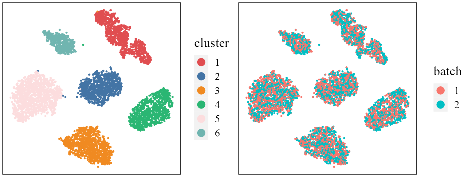
Combined differential epxression analysis
Finally, we condut the combined differential expression analysis using the integrated log-normalized expression matrix saved in the seuInt object. The function FindAllMarkers() in the Seurat R package is ued to achieve this analysis.
dat_deg <- FindAllMarkers(seuInt)
#> Calculating cluster 1
#> Calculating cluster 2
#> Calculating cluster 3
#> Calculating cluster 4
#> Calculating cluster 5
#> Calculating cluster 6
library(dplyr)
#> Warning: package 'dplyr' was built under R version 4.1.3
#>
#> Attaching package: 'dplyr'
#> The following objects are masked from 'package:stats':
#>
#>     filter, lag
#> The following objects are masked from 'package:base':
#>
#>     intersect, setdiff, setequal, union
n <- 5
dat_deg %>%
    group_by(cluster) %>%
    top_n(n = n, wt = avg_log2FC) -> top10
Plot dot plot of normalized expressions of the layer-specified marker genes for each spatial domain identified by using the FAST embeddings.
col_here <- c("#F2E6AB", "#9C0141")
library(ggplot2)
marker_Seurat <- readRDS("151507_DEGmarkerTop_5.rds")
marker_Seurat <- lapply(marker_Seurat, function(x) transferGeneNames(x, Method='eg.db'))
#> 'select()' returned 1:1 mapping between keys and columns
#> 'select()' returned 1:1 mapping between keys and columns
#> 'select()' returned 1:1 mapping between keys and columns
#> 'select()' returned 1:1 mapping between keys and columns
#> 'select()' returned 1:1 mapping between keys and columns
#> 'select()' returned 1:1 mapping between keys and columns
#> 'select()' returned 1:1 mapping between keys and columns
maker_genes <- unlist(lapply(marker_Seurat, toupper))
features <- maker_genes[!duplicated(maker_genes)]
p_dot <- DotPlot(seuInt, features=unname(features), cols=col_here, #  idents = ident_here,
              col.min = -1, col.max = 1) + coord_flip()+ theme(axis.text.y = element_text(face = "italic"))+
  ylab("Domain") + xlab(NULL) + theme(axis.text.x = element_text(size=12, angle = 25, hjust = 1, family='serif'),
                                      axis.text.y = element_text(size=12, face= "italic", family='serif'))
#> Warning in FetchData.Seurat(object = object, vars = features, cells = cells):
#> The following requested variables were not found: SNORC
p_dot
# table(unlist(yList), Idents(seuInt))Based on the marker genes, we annotate the Domains 1-9 as Layer5/6, Layer3/4, Layer5, Layer2/3, Layer2/3, Layer6, WM, Layer5, Layer1. Then, we rename the Domains using the function RenameIdents().
seuInt2 <- RenameIdents(seuInt, '1' = 'Layer6', '2' = 'Layer2/3', '3'="Layer5", '4'="WM",
                           '5'='Layer3/4', '6'= 'Layer1')
levels(seuInt2)  <- c("Layer1", "Layer2/3", "Layer3/4", "Layer5", "Layer6", "WM")
p_dot2 <- DotPlot(seuInt2, features=unname(features), cols=col_here, #  idents = ident_here,
              col.min = -1, col.max = 1) + coord_flip()+ theme(axis.text.y = element_text(face = "italic"))+
  ylab("Domain") + xlab(NULL) + theme(axis.text.x = element_text(size=12, angle = 25, hjust = 1, family='serif'),
                                      axis.text.y = element_text(size=12, face= "italic", family='serif'))
#> Warning in FetchData.Seurat(object = object, vars = features, cells = cells):
#> The following requested variables were not found: SNORC
p_dot2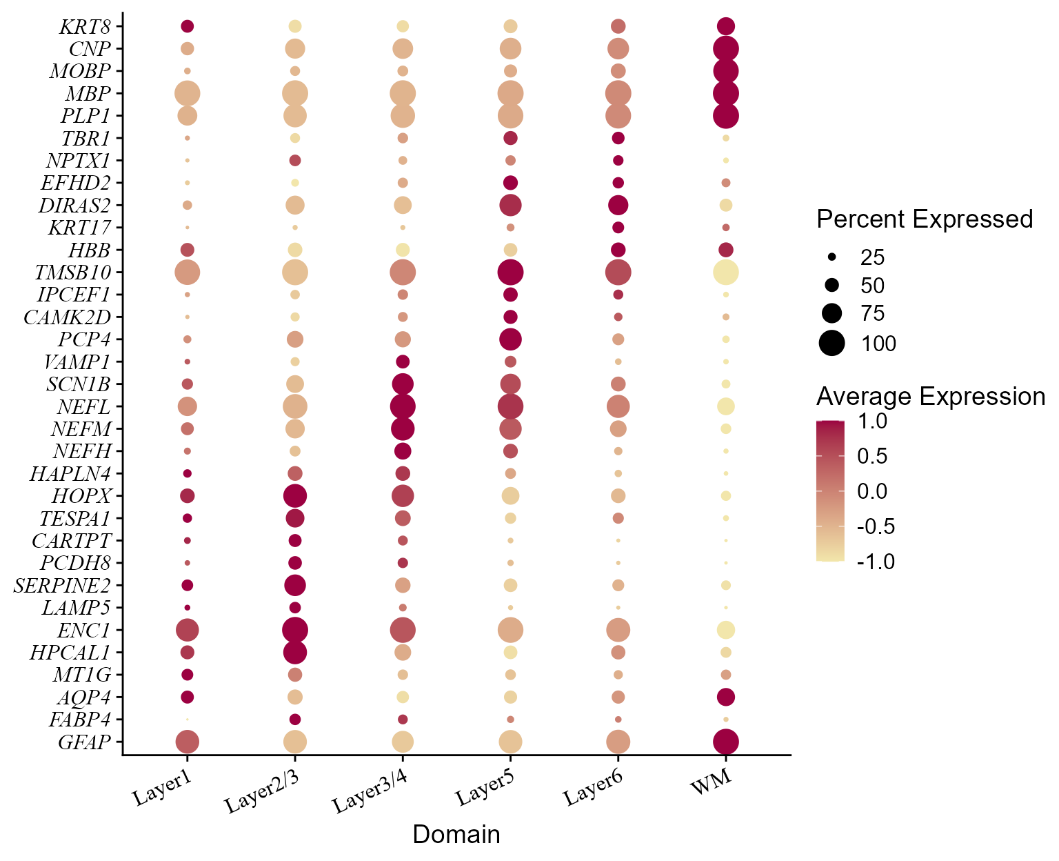
Session Info
sessionInfo()
#> R version 4.1.2 (2021-11-01)
#> Platform: x86_64-w64-mingw32/x64 (64-bit)
#> Running under: Windows 10 x64 (build 22621)
#>
#> Matrix products: default
#>
#> locale:
#> [1] LC_COLLATE=Chinese (Simplified)_China.936
#> [2] LC_CTYPE=Chinese (Simplified)_China.936
#> [3] LC_MONETARY=Chinese (Simplified)_China.936
#> [4] LC_NUMERIC=C
#> [5] LC_TIME=Chinese (Simplified)_China.936
#>
#> attached base packages:
#> [1] parallel  stats     graphics  grDevices utils     datasets  methods
#> [8] base
#>
#> other attached packages:
#> [1] dplyr_1.0.9        ggplot2_3.4.1      sp_1.5-0           SeuratObject_4.1.0
#> [5] Seurat_4.1.1       PRECAST_1.6.2      ProFAST_1.3        gtools_3.9.2.2
#>
#> loaded via a namespace (and not attached):
#>   [1] rappdirs_0.3.3              scattermore_0.8
#>   [3] ggthemes_4.2.4              GiRaF_1.0.1
#>   [5] ragg_1.2.2                  tidyr_1.2.0
#>   [7] bit64_4.0.5                 knitr_1.37
#>   [9] irlba_2.3.5                 DelayedArray_0.20.0
#>  [11] data.table_1.14.2           rpart_4.1.16
#>  [13] KEGGREST_1.34.0             RCurl_1.98-1.6
#>  [15] generics_0.1.2              BiocGenerics_0.40.0
#>  [17] org.Mm.eg.db_3.14.0         ScaledMatrix_1.2.0
#>  [19] cowplot_1.1.1               RSQLite_2.2.10
#>  [21] RANN_2.6.1                  future_1.26.1
#>  [23] bit_4.0.4                   spatstat.data_3.0-0
#>  [25] xml2_1.3.3                  httpuv_1.6.5
#>  [27] SummarizedExperiment_1.24.0 assertthat_0.2.1
#>  [29] viridis_0.6.2               xfun_0.29
#>  [31] hms_1.1.1                   jquerylib_0.1.4
#>  [33] evaluate_0.15               promises_1.2.0.1
#>  [35] fansi_1.0.4                 progress_1.2.2
#>  [37] dbplyr_2.1.1                igraph_1.3.5
#>  [39] DBI_1.1.2                   htmlwidgets_1.5.4
#>  [41] spatstat.geom_2.4-0         stats4_4.1.2
#>  [43] purrr_0.3.4                 ellipsis_0.3.2
#>  [45] RSpectra_0.16-1             ggpubr_0.4.0
#>  [47] backports_1.4.1             DR.SC_3.4
#>  [49] insight_0.17.0              biomaRt_2.50.3
#>  [51] deldir_1.0-6                sparseMatrixStats_1.6.0
#>  [53] MatrixGenerics_1.6.0        vctrs_0.6.1
#>  [55] SingleCellExperiment_1.16.0 Biobase_2.54.0
#>  [57] ROCR_1.0-11                 abind_1.4-5
#>  [59] cachem_1.0.6                withr_2.5.0
#>  [61] progressr_0.10.1            sctransform_0.3.3
#>  [63] prettyunits_1.1.1           mclust_5.4.10
#>  [65] goftest_1.2-3               cluster_2.1.2
#>  [67] lazyeval_0.2.2              crayon_1.5.1
#>  [69] pkgconfig_2.0.3             labeling_0.4.2
#>  [71] GenomeInfoDb_1.30.1         nlme_3.1-155
#>  [73] vipor_0.4.5                 nnet_7.3-17
#>  [75] rlang_1.1.0                 globals_0.15.0
#>  [77] lifecycle_1.0.3             miniUI_0.1.1.1
#>  [79] filelock_1.0.2              BiocFileCache_2.2.1
#>  [81] rsvd_1.0.5                  rprojroot_2.0.3
#>  [83] polyclip_1.10-0             matrixStats_0.62.0
#>  [85] lmtest_0.9-40               Matrix_1.4-0
#>  [87] carData_3.0-5               zoo_1.8-10
#>  [89] beeswarm_0.4.0              ggridges_0.5.3
#>  [91] png_0.1-7                   viridisLite_0.4.1
#>  [93] bitops_1.0-7                KernSmooth_2.23-20
#>  [95] Biostrings_2.62.0           blob_1.2.2
#>  [97] DelayedMatrixStats_1.16.0   stringr_1.4.0
#>  [99] parallelly_1.32.0           spatstat.random_2.2-0
#> [101] rstatix_0.7.0               S4Vectors_0.32.3
#> [103] ggsignif_0.6.3              beachmat_2.10.0
#> [105] scales_1.2.1                memoise_2.0.1
#> [107] magrittr_2.0.3              plyr_1.8.7
#> [109] ica_1.0-2                   zlibbioc_1.40.0
#> [111] compiler_4.1.2              RColorBrewer_1.1-3
#> [113] fitdistrplus_1.1-8          cli_3.2.0
#> [115] XVector_0.34.0              listenv_0.8.0
#> [117] patchwork_1.1.1             pbapply_1.5-0
#> [119] MASS_7.3-55                 mgcv_1.8-39
#> [121] tidyselect_1.1.2            stringi_1.7.6
#> [123] textshaping_0.3.6           highr_0.9
#> [125] yaml_2.3.6                  BiocSingular_1.10.0
#> [127] ggrepel_0.9.1               grid_4.1.2
#> [129] sass_0.4.1                  tools_4.1.2
#> [131] future.apply_1.9.0          rstudioapi_0.13
#> [133] gridExtra_2.3               farver_2.1.1
#> [135] Rtsne_0.16                  digest_0.6.29
#> [137] rgeos_0.5-9                 shiny_1.7.1
#> [139] Rcpp_1.0.10                 GenomicRanges_1.46.1
#> [141] car_3.0-12                  broom_0.7.12
#> [143] scuttle_1.4.0               performance_0.8.0
#> [145] later_1.3.0                 harmony_0.1.0
#> [147] RcppAnnoy_0.0.19            org.Hs.eg.db_3.14.0
#> [149] httr_1.4.3                  AnnotationDbi_1.56.2
#> [151] colorspace_2.1-0            XML_3.99-0.9
#> [153] fs_1.5.2                    tensor_1.5
#> [155] reticulate_1.25             IRanges_2.28.0
#> [157] splines_4.1.2               uwot_0.1.11
#> [159] spatstat.utils_3.0-1        pkgdown_2.0.6
#> [161] scater_1.25.1               plotly_4.10.0
#> [163] systemfonts_1.0.4           xtable_1.8-4
#> [165] jsonlite_1.8.0              R6_2.5.1
#> [167] pillar_1.9.0                htmltools_0.5.2
#> [169] mime_0.12                   glue_1.6.2
#> [171] fastmap_1.1.0               BiocParallel_1.28.3
#> [173] BiocNeighbors_1.12.0        codetools_0.2-18
#> [175] utf8_1.2.3                  lattice_0.20-45
#> [177] bslib_0.3.1                 spatstat.sparse_2.1-1
#> [179] tibble_3.2.1                curl_4.3.2
#> [181] ggbeeswarm_0.6.0            leiden_0.4.2
#> [183] limma_3.50.1                survival_3.2-13
#> [185] CompQuadForm_1.4.3          rmarkdown_2.11
#> [187] desc_1.4.0                  munsell_0.5.0
#> [189] GenomeInfoDbData_1.2.7      reshape2_1.4.4
#> [191] gtable_0.3.3                spatstat.core_2.4-4